Fast disconnected ICAR in Stan

Using the segment feature in Stan to implement the ICAR model

Note: actually, Mitzi already got to this – see here for her version!

Introduction

Morris et al. (2019) provide a (more) efficient implementation of the intrinsic conditional auto-regressive (ICAR) model in Stan. In this post I extend their approach to the case when the adjacency graph is disconnected, using Section 8.2. of the Stan User’s Guide for indexing. Their paper follows from the Spatial Models in Stan: Intrinsic Auto-Regressive Models for Areal Data case study which I’d recommend having a look at.

Background

Consider areas \(\{A_i\}_{i = 1, \ldots, n}\) with corresponding spatial random effects \(\boldsymbol{\phi} = (\phi_1, \ldots, \phi_n)^\top\) distributed according to the zero-mean intrinsic Gaussian Markov random field \[ \boldsymbol{\phi} \sim \mathcal{N}(\mathbf{0}, \tau_\phi^{-1} \mathbf{R}^{-}), \label{eq:gmrf}, \] where \(\tau_\phi\) is the precision and \(\mathbf{R}^{-}\) is the pseudo-inverse of the rank-deficient structure matrix \(\mathbf{R}\) (such that the precision matrix is given by \(\tau_\phi \mathbf{R}\)). One way to specify the structure matrix is by the Laplacian of the adjacency graph \(\mathcal{G} = (\mathcal{V}, \mathcal{E})\), with \(n\) vertices \(v \in \mathcal{V}\) corresponding to each area and edges \(e \in \mathcal{E}\) between vertices \(i\) and \(j\) when areas are adjacent, denoted \(i \sim j\). This results in an improper density \[ p(\boldsymbol{\phi}) \propto \exp \left( -\frac{\tau_\phi}{2} \boldsymbol{\phi}^\top \mathbf{R} \boldsymbol{\phi} \right), \] so called because it is invariant to certain linear transformations of \(\boldsymbol{\phi}\).

Two important issues when working with these types of models are:

• Scaling the structure matrix In order for \(\tau_\phi\) to have a consistent interpretation across models, the structure matrix \(\mathbf{R}\) (which is a function of the adjacency graph) requires scaling. This “consistent interpretation across models” is useful when you are setting priors, among other things. When \(\tau_\phi = 1\) we would like the “typical marginal variance” to be one as well. This requires scaling the structure matrix, say replacing it with a scaled version \(\mathbf{R}^\star\).

• Constraining the spatial random effects So that the random effect can be identified we place constraints on \(\boldsymbol{\phi}\). It is standard (for example in R-INLA) to use sum-to-zero constraints of the form \(\sum_i \phi_i = 0\).

Particular care is required when \(\mathcal{G}\) is disconnected (a graph is disconnceted when there exist areas which can’t be reached following the vertices of the adjacency graph.) For this reason Morris et al. (2019) consider only connected graphs, stating that the indexing required in the disconnected case would complicate the code for presentation purposes. In some settings the graph is disconnected and there is little that can be done about it. Hopefully this post provides a starting point.

Recommendations for dealing scaling and constraints in the disconnected case are given by Freni-Sterrantino, Ventrucci, and Rue (2018). To summarise, they firstly recommend to scale local smoothing in each connected component independently so that τϕ has a consistent interpretation within the model. Secondly, they recommend to place a sum-to-zero constraint on each connected component made up of at least two areas. This results in “singletons” having independent zero-mean Gaussian random effects (rather than constraining them to be identically zero which is another possible choice).

Example implementation

library(bsae)
library(dplyr)
library(ggplot2)
library(rstan)

Malawi (if you attend Imperial’s HIV inference group meetings you’ll know that this is the only country which exists) has 28 districts and one of them, Likoma is an island – or singleton.

bsae is a personal package I am working on which contains the simple features dataframe mw which has data about HIV cases mw$y and sample sizes mw$n_obs in Malawi from a particular survey. A neighbours object can be extracted from the geometry mw$geometry giving:

nb <- sf_to_nb(mw)
nb

Neighbour list object:
Number of regions: 28 
Number of nonzero links: 108 
Percentage nonzero weights: 13.77551 
Average number of links: 3.857143 
1 region with no links:
2

As you can see there is one region, Likoma, with no links. nb can be used to create the unscaled structure matrix:

R <- nb_to_precision(nb)
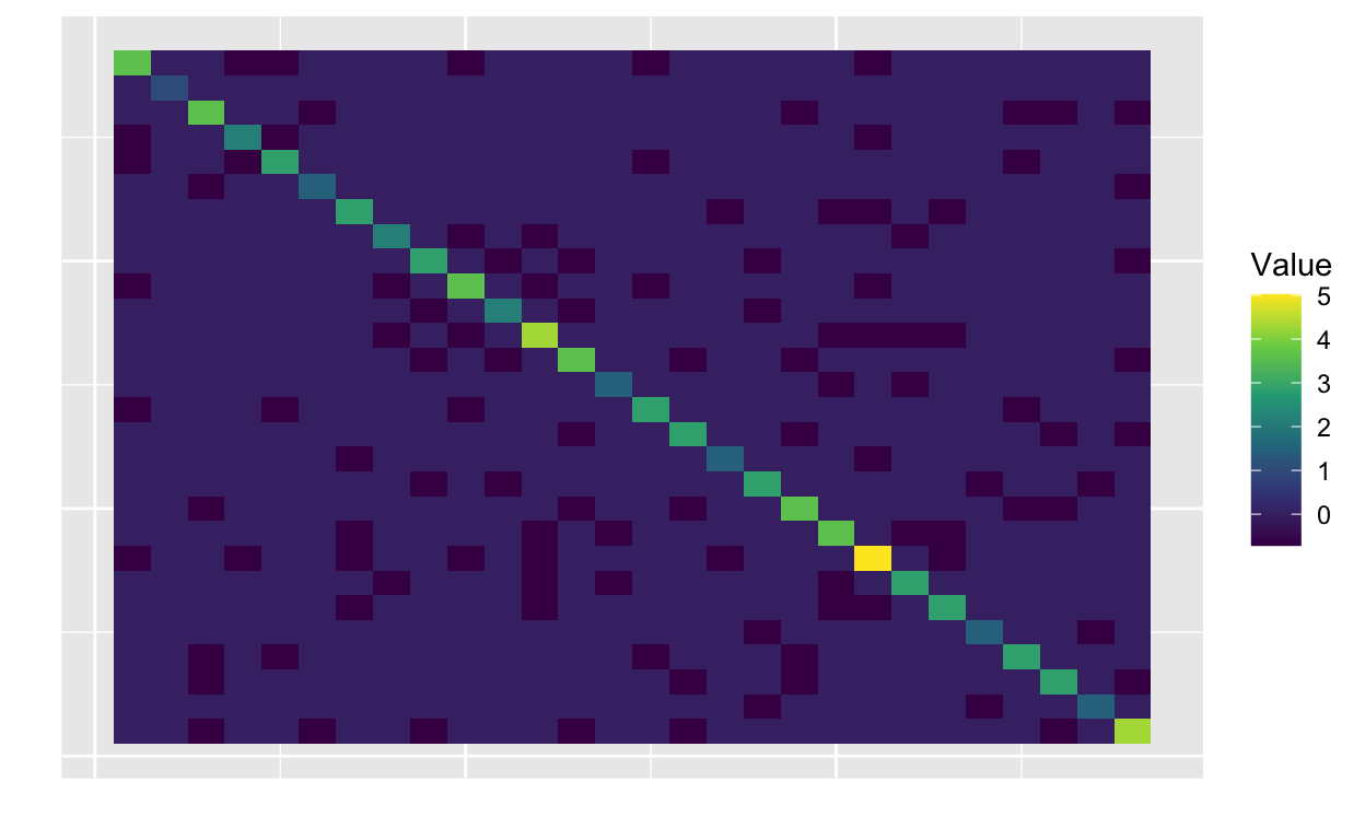
plot_matrix(R)

In the second row and column, all of the values are zero. In particular, the entry R[2, 2] is zero giving \(\phi_2\) infinite variance according to the unscaled prior! Using scale_grmf_precision replaces this value by one such that \(\phi_2 \sim \mathcal{N}(0, \tau_\phi^{-1})\) as well as scaling the submatrix corresponding to the mainland such that the mean of the marginal variances is one.

R_scaled <- scale_gmrf_precision(R)
plot_matrix(R_scaled$Q)

The matrix R_scaled$Q is very similar to R, just with a different value at [2, 2] and the rest of the matrix rescaled.

I will now fit a Bayesian hierarchical model to the case data, using a ICAR spatial random effect model following Morris et al. (2019), making some adjustments to deal with the disconnected graph.

To pass Stan information about the connected components I use three entries in the data block:

• nc, the number of connected components, nc = 2 in this case
• group_sizes, a vector of length nc giving the number of areas within each connected component, group_sizes = c(27, 1) here
• scales, a vector of length n used to rescale the GMRF

The Stan code for the model is:

data {
  int<lower=1> n; // Number of regions
  int y[n];       // Vector of responses
  int m[n];       // Vector of sample sizes
  
  // Data structure for connected components input
  int<lower=1> nc;
  int group_sizes[nc];    
  vector[n] scales;
  
  // Data structure for graph input
  int<lower=1> n_edges;
  int<lower=1, upper=n> node1[n_edges];
  int<lower=1, upper=n> node2[n_edges];
}

parameters {
  real beta_0;             // Intercept
  vector[n] u;             // Unscaled spatial effects
  real<lower=0> sigma_phi; // Standard deviation of spatial effects
}

transformed parameters {
  real tau_phi = 1 / sigma_phi^2; // Precision of spatial effects
}

model {
  // ICAR model
  int pos;
  pos = 1;
  for (k in 1:nc) {
  
    if(group_sizes[k] == 1){
      // Independent unit normal prior on singletons
      segment(u, pos, group_sizes[k]) ~ normal(0, 1);
    }
    
    if(group_sizes[k] > 1){
      // Soft sum-to-zero constraint on 
      // each non-singleton connected component
      sum(segment(u, pos, group_sizes[k])) ~ normal(0, 0.001 * group_sizes[k]);
    }
    
    pos = pos + group_sizes[k];
  }
  // Note that the below increment doesn't feature singletons
  target += -0.5 * dot_self(u[node1] - u[node2]);
  
  // The rest of the model
  y ~ binomial_logit(m, beta_0 + sigma_phi * sqrt(1 ./ scales) .* u);
  beta_0 ~ normal(-2, 1);
  sigma_phi ~ normal(0, 2.5);
}

generated quantities {
  vector[n] phi = sigma_phi * sqrt(1 ./ scales) .* u;
  vector[n] rho = inv_logit(beta_0 + phi);
}

The most interesting part is the ICAR prior in the model block.

I have used the segment operation to implement a ragged data structure (the number of areas in each connected component) following the Stan User’s Guide. Because u is arranged with the connected components grouped together, segment(u, 1, group_sizes[1]) gives all of the mainland and segment(u, 27, group_sizes[2]) gives Likoma. The expression

sum(segment(u, pos, group_sizes[k])) ~ normal(0, 0.001 * group_sizes[k])

specifies that the mean of the segment is approximately zero. Morris et al. (2019) find that this type of “soft constraint” works better than a hard constraint where the sum must be identically zero.

One complication is that using this Stan code requires reordering the data so that the connected components are grouped together. In the case of mw this just involves moving Likoma from the second row to the last, though in general there may be more shuffling.

comp <- spdep::n.comp.nb(nb)
comp

$nc
[1] 2

$comp.id
 [1] 1 2 1 1 1 1 1 1 1 1 1 1 1 1 1 1 1 1 1 1 1 1 1 1 1 1 1 1

ordered_mw <- mw %>%
  mutate(comp.id = comp$comp.id) %>%
  arrange(comp.id)

I create the graph inputs as follows:

ordered_nb <- sf_to_nb(ordered_mw)
ordered_g <- nb_to_graph(ordered_nb)

And the three inputs used to specify the connected components are:

ordered_comp <- spdep::n.comp.nb(ordered_nb)
ordered_comp$nc

[1] 2

rle <- rle(ordered_comp$comp.id) #' Run length encoding 
rle

Run Length Encoding
  lengths: int [1:2] 27 1
  values : int [1:2] 1 2

ordered_scales <- ordered_nb %>%
  nb_to_precision() %>%
  scale_gmrf_precision()

vec_scales <- ordered_scales$scales[ordered_comp$comp.id]
vec_scales

 [1] 0.7171335 0.7171335 0.7171335 0.7171335 0.7171335 0.7171335
 [7] 0.7171335 0.7171335 0.7171335 0.7171335 0.7171335 0.7171335
[13] 0.7171335 0.7171335 0.7171335 0.7171335 0.7171335 0.7171335
[19] 0.7171335 0.7171335 0.7171335 0.7171335 0.7171335 0.7171335
[25] 0.7171335 0.7171335 0.7171335 1.0000000

vec_scales contains the scaling constant 0.7171335 for the mainland and the value 1 for Likoma. In some sense, really the scaling constant for the island should be Inf, but as you can see in the Stan code we are treating it with a special case (and so don’t want to do alter the scaling).

Now I can pass the data to Stan and start sampling:

#' A quirk of the data I'm using is that counts might not be integers
#' This is because of survey weighting

dat <- list(
  n = nrow(ordered_mw),
  y = round(ordered_mw$y),  
  m = round(ordered_mw$n_obs),
  nc = comp$nc,
  group_sizes = rle$lengths,
  scales = vec_scales,
  n_edges = ordered_g$n_edges,
  node1 = ordered_g$node1,
  node2 = ordered_g$node2
)

stan_fit <- rstan::sampling(fast_disconnected, data = dat, warmup = 500, iter = 1000)
out <- rstan::extract(stan_fit)

rstan::summary(stan_fit)$summary[c("beta_0", "phi[28]"), ]

               mean     se_mean         sd       2.5%         25%
beta_0  -2.48623132 0.000741430 0.03695507 -2.5584735 -2.51154357
phi[28]  0.03156711 0.003721093 0.18387424 -0.3326178 -0.08825791
                50%        75%      97.5%    n_eff      Rhat
beta_0  -2.48548249 -2.4615027 -2.4148429 2484.322 0.9990385
phi[28]  0.03692491  0.1582221  0.3862023 2441.748 0.9987896

There is more exploring to do here!

Conclusion

To test if this worked I should evaluate it in comparison to a version fitted with R-INLA. Along the lines of:

dat <- list(id = 1:nrow(ordered_mw),
             y = round(ordered_mw$y),
             m = round(ordered_mw$n_obs))

tau_prior <- list(prec = list(prior = "logtnormal", param = c(0, 1 / 2.5^2),
                              initial = 0, fixed = FALSE))

formula <- y ~ 1 + f(id,
                     model = "besag",
                     graph = nb,
                     scale.model = TRUE,
                     constr = TRUE,
                     hyper = tau_prior)

inla_fit <- INLA::inla(formula,
                       family = "binomial",
                       control.family = list(control.link = list(model = "logit")),
                       data = dat,
                       Ntrials = m,
                       control.predictor = list(compute = TRUE, link = 1),
                       control.compute = list(dic = TRUE, waic = TRUE,
                                              cpo = TRUE, config = TRUE))

That being said, I have found it often tricky to get Stan and R-INLA to agree!