A Models for areal spatial structure

A.1 Comparison of AGHQ to NUTS

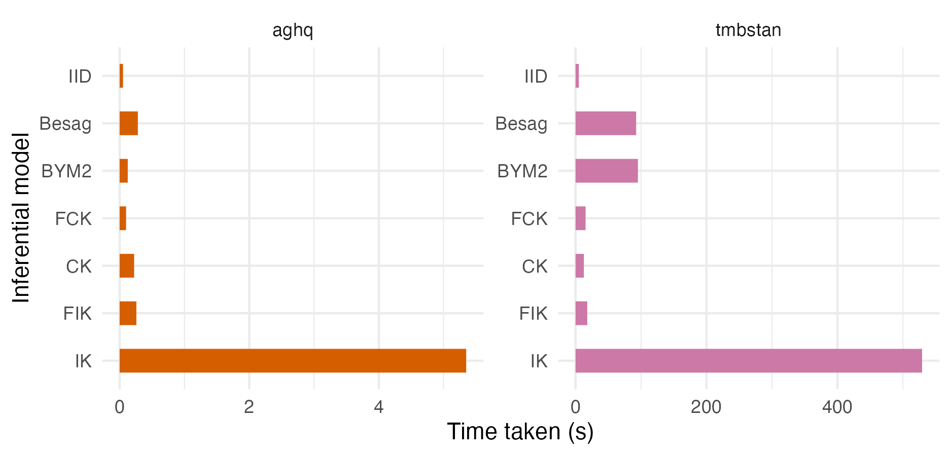
A comparison of time taken to fit AGHQ via aghq as compared with NUTS via tmbstan for each inferential model. For the models run using NUTS via tmbstan there was significant variation in time taken depending on initial random seed. As such, these timings and more broadly the inferences obtained from NUTS in Appendix A.1 should be interpreted with appropriate skepticism.

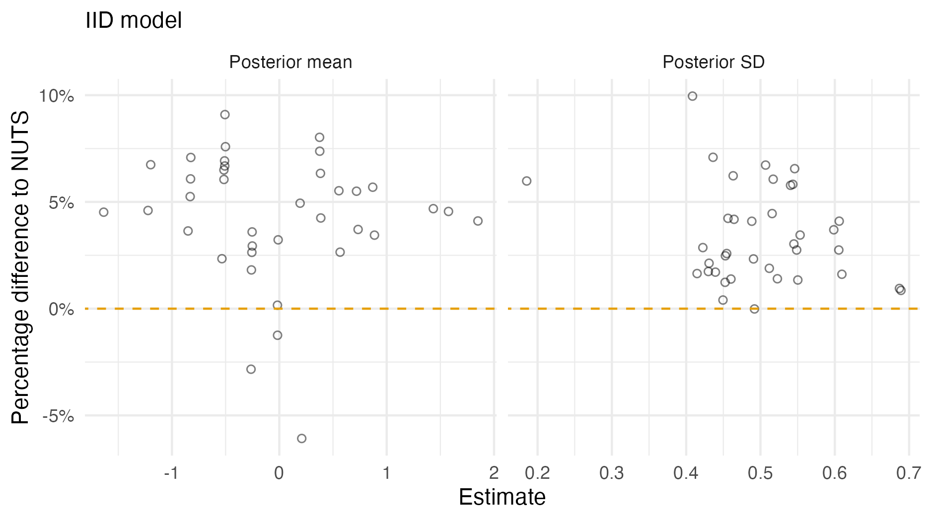
Figure A.1: A comparison of time taken to fit AGHQ via aghq as compared with NUTS via tmbstan for each inferential model. For the models run using NUTS via tmbstan there was significant variation in time taken depending on initial random seed. As such, these timings and more broadly the inferences obtained from NUTS in Appendix A.1 should be interpreted with appropriate skepticism.

A comparison of the posterior means and standard deviations obtained with AGHQ via aghq as compared with NUTS via tmbstan fitting an IID inferential model to IID synthetic data on the grid geometry (Panel 4.6E). For NUTS, the minimum ESS was 1686, and the maximum value of the potential scale reduction factor was 1.00.

Figure A.2: A comparison of the posterior means and standard deviations obtained with AGHQ via aghq as compared with NUTS via tmbstan fitting an IID inferential model to IID synthetic data on the grid geometry (Panel 4.6E). For NUTS, the minimum ESS was 1686, and the maximum value of the potential scale reduction factor was 1.00.

A comparison of the posterior means and standard deviations obtained with AGHQ via aghq as compared with NUTS via tmbstan fitting a Besag inferential model to IID synthetic data on the grid geometry (Panel 4.6E). For NUTS, the minimum ESS was 1056, and the maximum value of the potential scale reduction factor was 1.00.

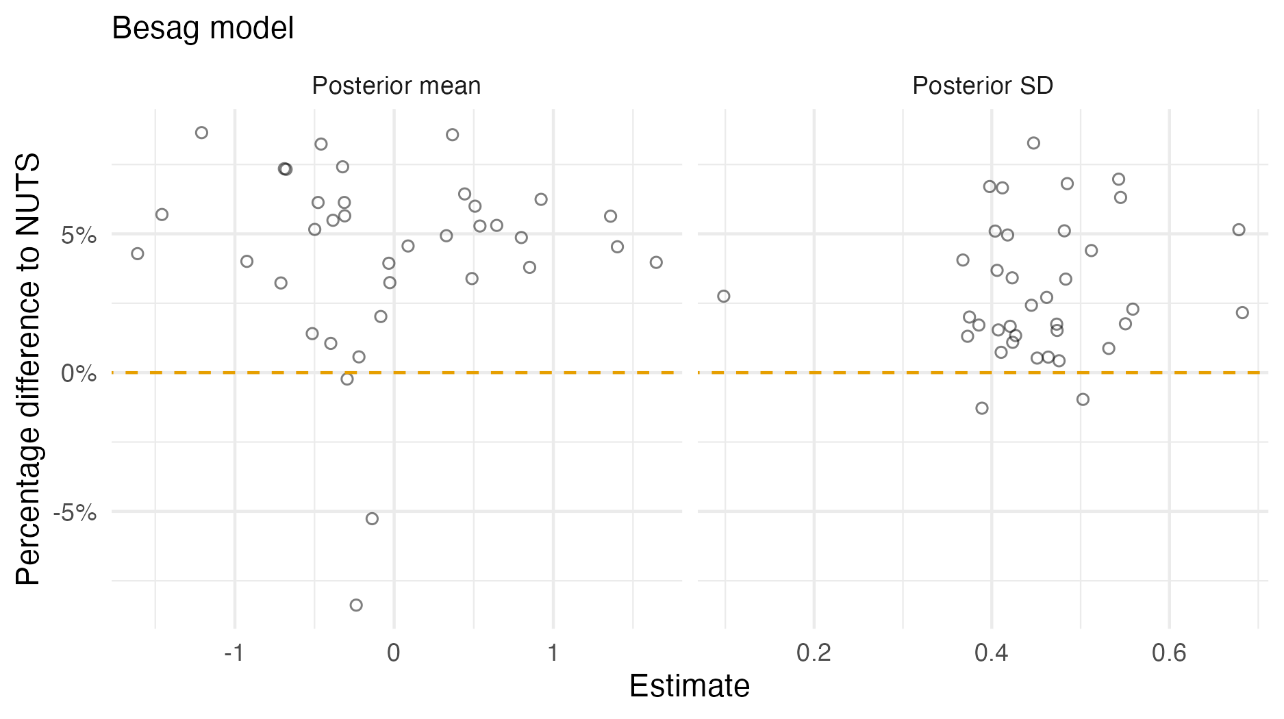
Figure A.3: A comparison of the posterior means and standard deviations obtained with AGHQ via aghq as compared with NUTS via tmbstan fitting a Besag inferential model to IID synthetic data on the grid geometry (Panel 4.6E). For NUTS, the minimum ESS was 1056, and the maximum value of the potential scale reduction factor was 1.00.

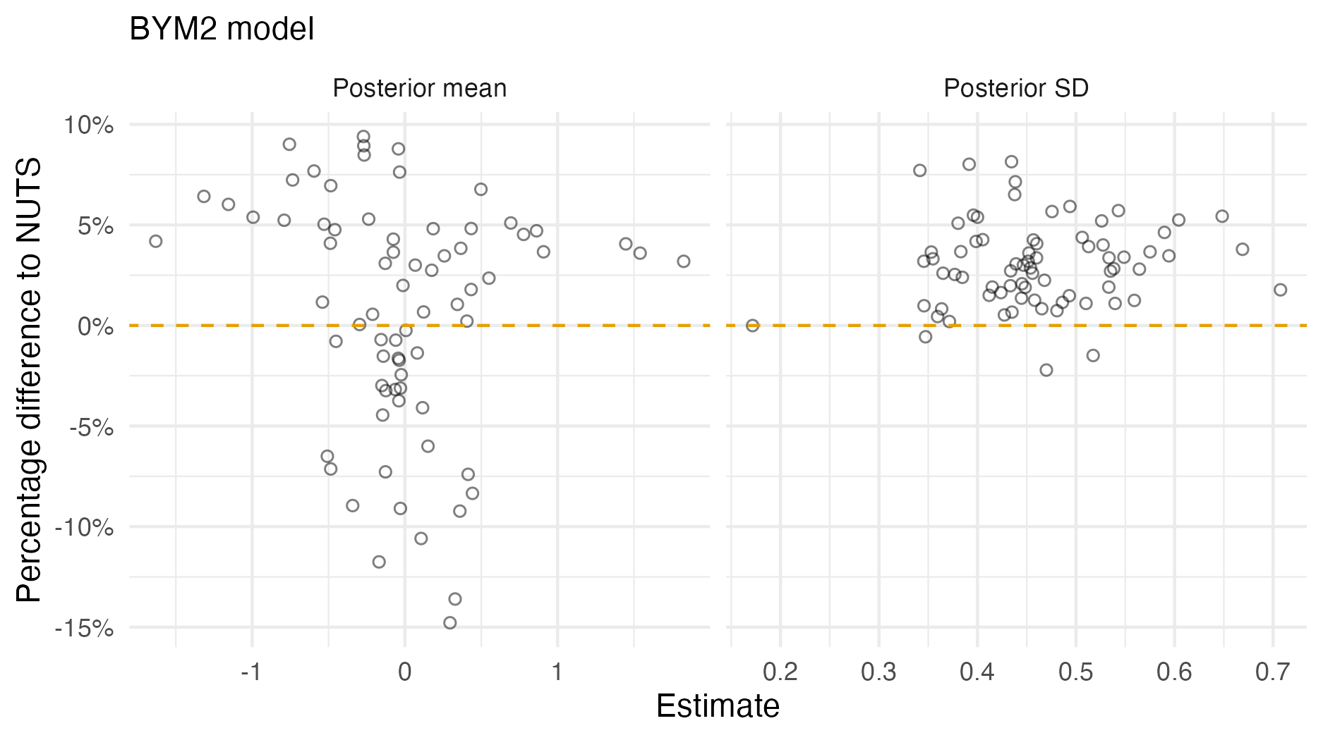
A comparison of the posterior means and standard deviations obtained with AGHQ via aghq as compared with NUTS via tmbstan fitting a BYM2 inferential model to IID synthetic data on the grid geometry (Panel 4.6E). For NUTS, the minimum ESS was 35, and the maximum value of the potential scale reduction factor was 1.06.

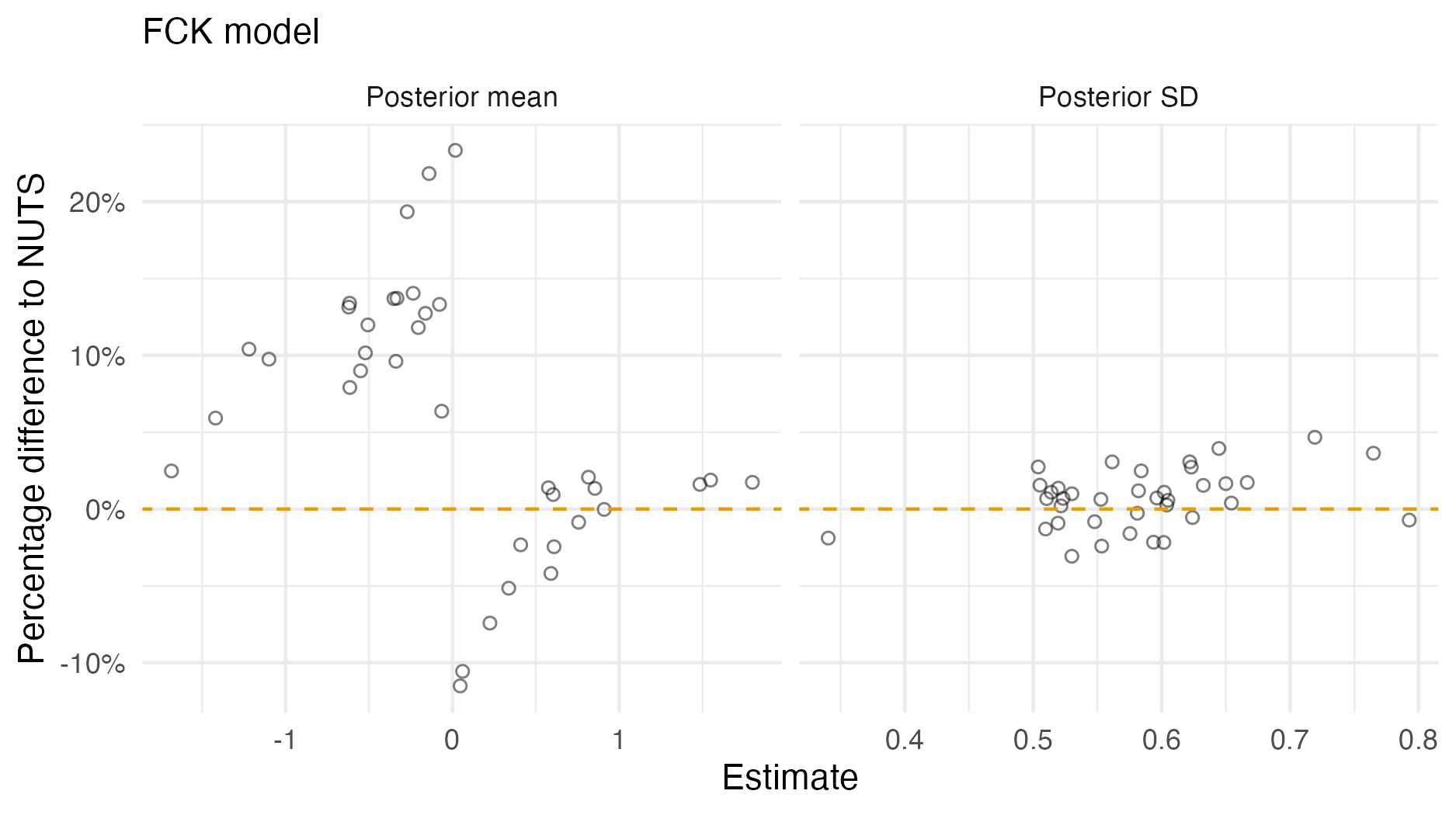
Figure A.4: A comparison of the posterior means and standard deviations obtained with AGHQ via aghq as compared with NUTS via tmbstan fitting a BYM2 inferential model to IID synthetic data on the grid geometry (Panel 4.6E). For NUTS, the minimum ESS was 35, and the maximum value of the potential scale reduction factor was 1.06.

A comparison of the posterior means and standard deviations obtained with AGHQ via aghq as compared with NUTS via tmbstan fitting a FCK inferential model to IID synthetic data on the grid geometry (Panel 4.6E). For NUTS, the minimum ESS was 355, and the maximum value of the potential scale reduction factor was 1.01.

Figure A.5: A comparison of the posterior means and standard deviations obtained with AGHQ via aghq as compared with NUTS via tmbstan fitting a FCK inferential model to IID synthetic data on the grid geometry (Panel 4.6E). For NUTS, the minimum ESS was 355, and the maximum value of the potential scale reduction factor was 1.01.

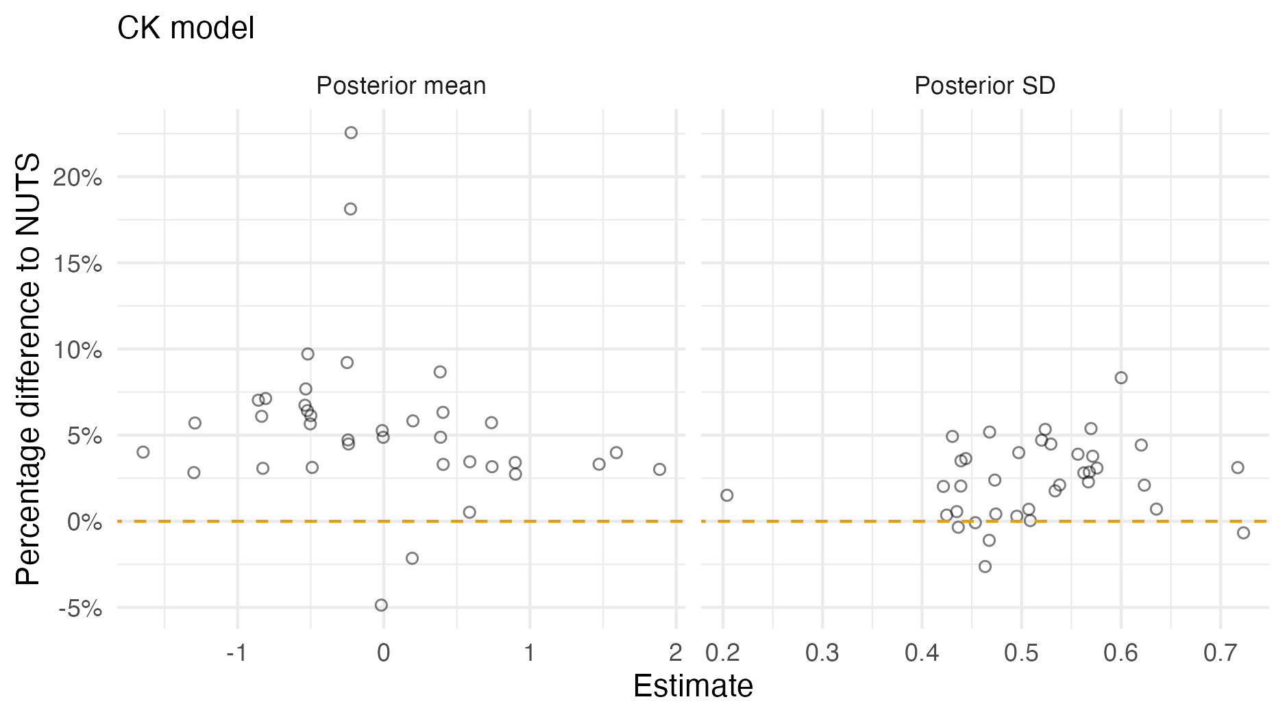
A comparison of the posterior means and standard deviations obtained with AGHQ via aghq as compared with NUTS via tmbstan fitting a CK inferential model to IID synthetic data on the grid geometry (Panel 4.6E). For NUTS, the minimum ESS was 1471, and the maximum value of the potential scale reduction factor was 1.00.

Figure A.6: A comparison of the posterior means and standard deviations obtained with AGHQ via aghq as compared with NUTS via tmbstan fitting a CK inferential model to IID synthetic data on the grid geometry (Panel 4.6E). For NUTS, the minimum ESS was 1471, and the maximum value of the potential scale reduction factor was 1.00.

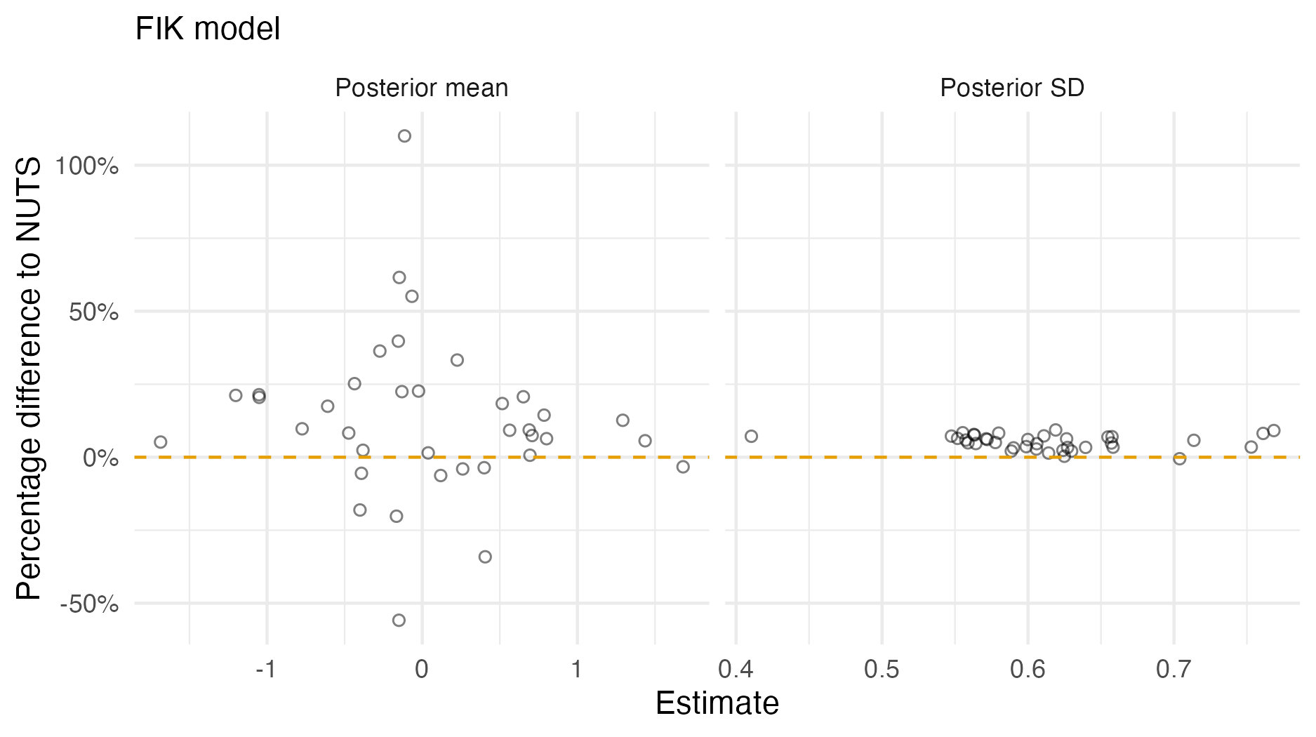
A comparison of the posterior means and standard deviations obtained with AGHQ via aghq as compared with NUTS via tmbstan fitting a FIK inferential model to IID synthetic data on the grid geometry (Panel 4.6E). For NUTS, the minimum ESS was 289, and the maximum value of the potential scale reduction factor was 1.01.

Figure A.7: A comparison of the posterior means and standard deviations obtained with AGHQ via aghq as compared with NUTS via tmbstan fitting a FIK inferential model to IID synthetic data on the grid geometry (Panel 4.6E). For NUTS, the minimum ESS was 289, and the maximum value of the potential scale reduction factor was 1.01.

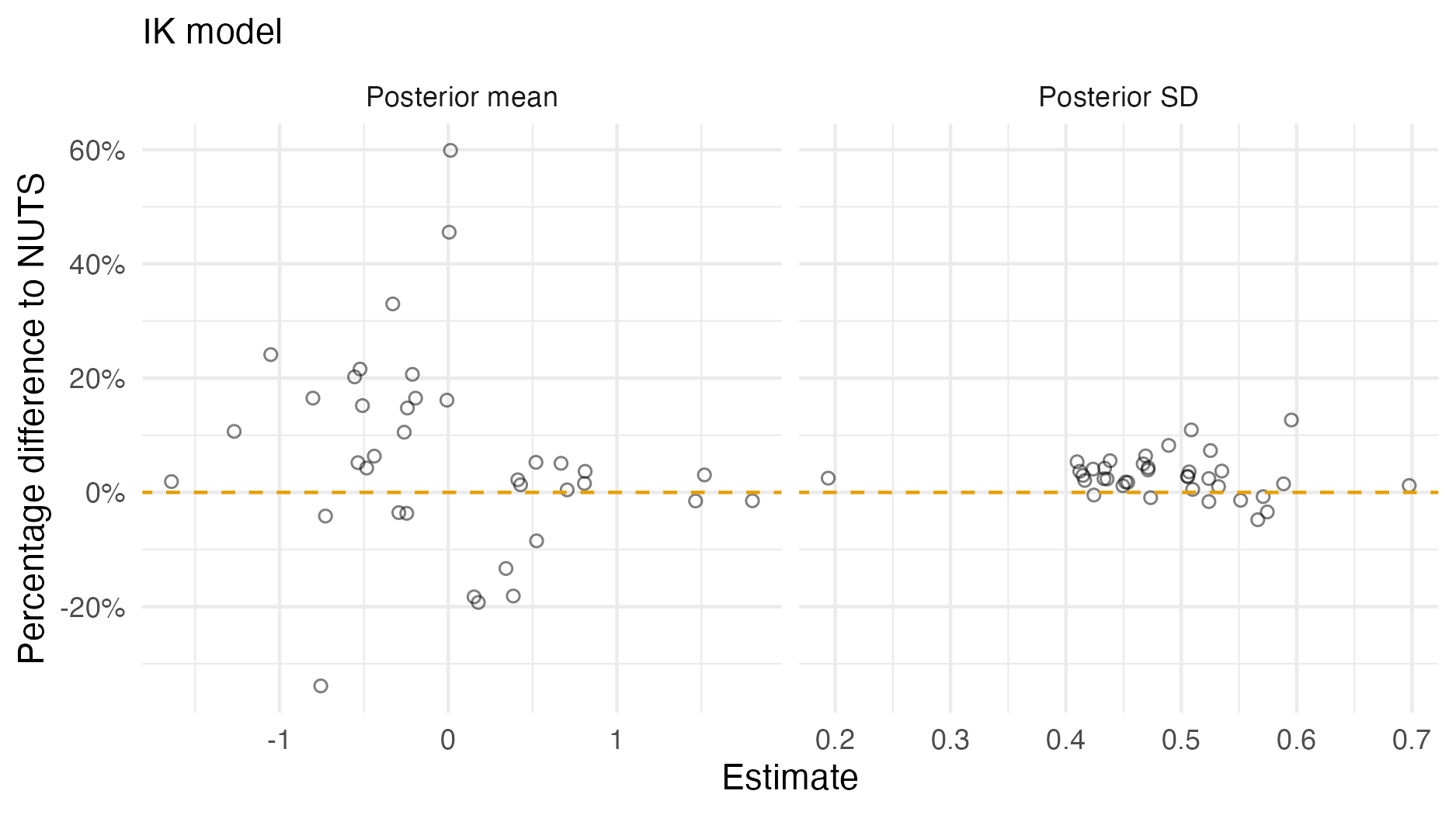
A comparison of the posterior means and standard deviations obtained with AGHQ via aghq as compared with NUTS via tmbstan fitting a IK inferential model to IID synthetic data on the grid geometry (Panel 4.6E). For NUTS, the minimum ESS was 1623, and the maximum value of the potential scale reduction factor was 1.00.

Figure A.8: A comparison of the posterior means and standard deviations obtained with AGHQ via aghq as compared with NUTS via tmbstan fitting a IK inferential model to IID synthetic data on the grid geometry (Panel 4.6E). For NUTS, the minimum ESS was 1623, and the maximum value of the potential scale reduction factor was 1.00.

A.2 Lengthscale prior sensitivity

Table A.1: Six lengthscale prior distributions were considered for use in the simulation (Section 4.3) and HIV prevalence (Section 4.4) studies.
Description	Prior	Additional details
Gamma	$l \sim \text{Gamma}(1, 1)$	$-$
Geometry-informed inverse-gamma	$l \sim \text{IG}(a, b)$	The parameters $a$ and $b$ chosen such that 5% of the prior mass was below and above the 5% and 95% quantile for distance between points (Betancourt 2017)
Geometry-informed normal	$l \sim \mathcal{N}^{+}(0, \sigma)$	The parameter $\sigma$ set as one third the difference between the minimum and maximum distance between points (Betancourt 2017)
Log-normal	$l \sim \text{Log-normal}(0, 1)$	$-$
Non-informative	$p(l) = 1$	This is an improper prior in that it does not integrate to one
Oracle normal	$l \sim \mathcal{N}^{+}(2.5, 1)$	The mean of this prior was set to the true value of the lengthscale

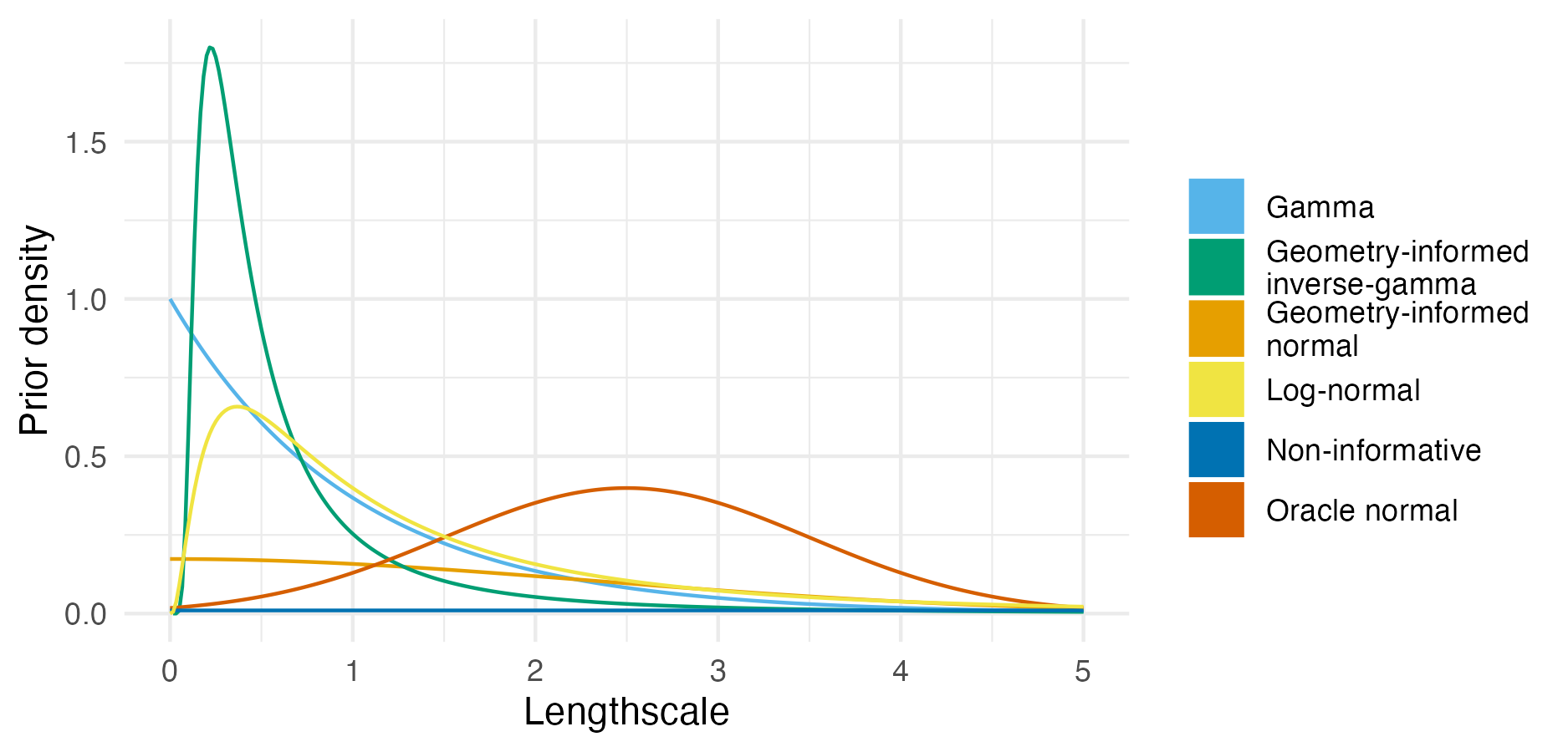
Figure A.9: The probability density for each lengthscale prior distribution as given in Table A.1.

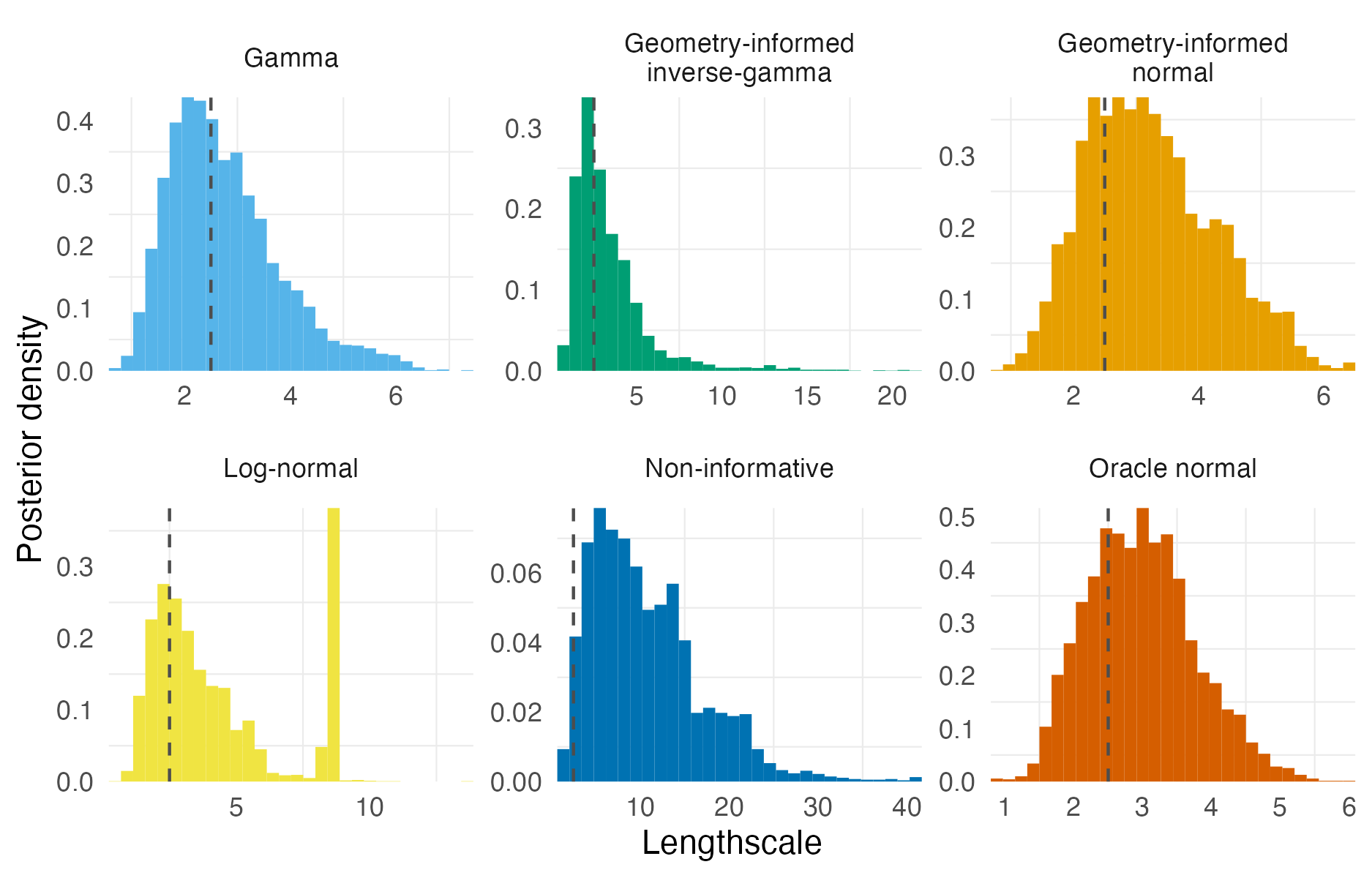
Lengthscale posterior distributions obtained using NUTS to fit a centroid kernel model to integrated kernel data. The true value, 2.5, is shown as a dashed vertical line. Six different lengthscale prior distributions were considered as given in Table A.1. The geometry used was the grid (Panel 4.6E).

Figure A.10: Lengthscale posterior distributions obtained using NUTS to fit a centroid kernel model to integrated kernel data. The true value, 2.5, is shown as a dashed vertical line. Six different lengthscale prior distributions were considered as given in Table A.1. The geometry used was the grid (Panel 4.6E).

A.3 Simulation study

A.3.1 Lengthscale recovery

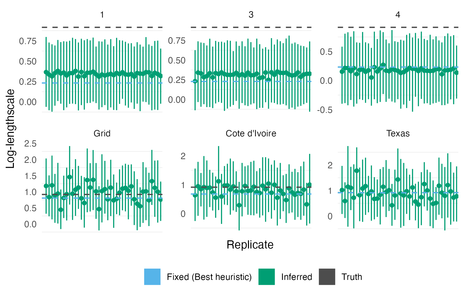
The lengthscale posterior mean and 95% credible interval obtained using the centroid kernel model on integrated kernel data for the first 40 simulation replicates on each geometry. The true lengthscale, and lengthscale obtained using the heuristic method of N. Best et al. (1999), are shown as dashed horizontal lines.

Figure A.11: The lengthscale posterior mean and 95% credible interval obtained using the centroid kernel model on integrated kernel data for the first 40 simulation replicates on each geometry. The true lengthscale, and lengthscale obtained using the heuristic method of N. Best et al. (1999), are shown as dashed horizontal lines.

A.3.2 BYM2 proportion

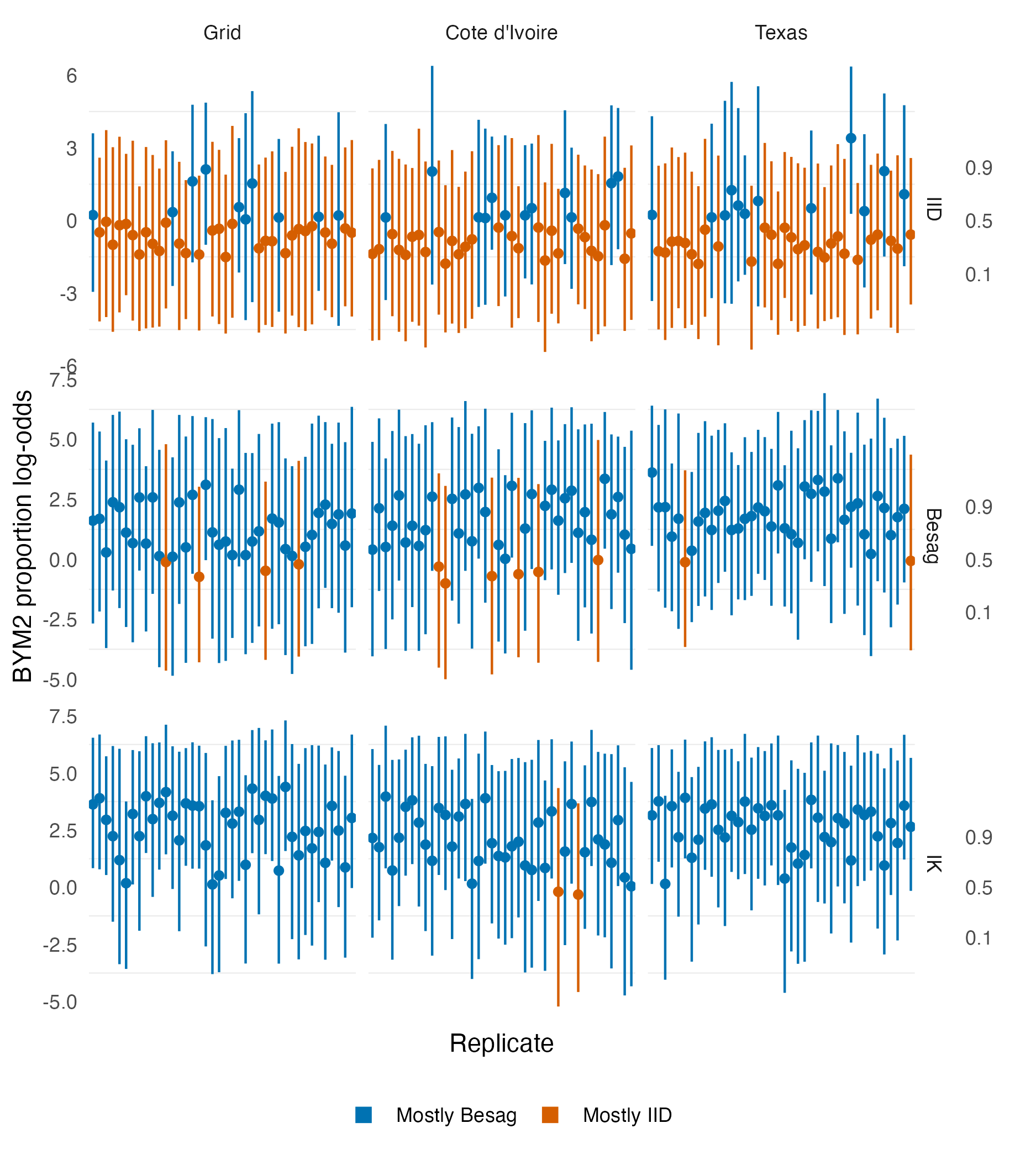
The BYM2 proportion parameter posterior mean and 95% credible interval obtained for the first 40 simulation replicates for the realistic geometries. When the simulated data is IID, the BYM2 proportion parameter is in the majority of cases below 0.5, corresponding to have inferred that the noise is mostly IID (spatially unstructured) When the simulated data is either Besag or IK, the BYM2 proportion parameter is in the majority of cases above 0.5, corresponding to have inferred that the noise is mostly Besag (spatially structured).

Figure A.12: The BYM2 proportion parameter posterior mean and 95% credible interval obtained for the first 40 simulation replicates for the realistic geometries. When the simulated data is IID, the BYM2 proportion parameter is in the majority of cases below 0.5, corresponding to have inferred that the noise is mostly IID (spatially unstructured) When the simulated data is either Besag or IK, the BYM2 proportion parameter is in the majority of cases above 0.5, corresponding to have inferred that the noise is mostly Besag (spatially structured).

A.3.3 Mean squared error

Table A.2: The average mean squared error (MSE) of each inferential model in estimating $\rho$, under different simulation and geometry settings. Entries for FCK and CK on geometry 2 are empty because model was undefined in that case. The units used in this table are thousandths.
Simulation model	Inferential model
Simulation model	IID	Besag	BYM2	FCK	CK	FIK	IK
1
IID	8.20	7.56	7.99	7.84	7.67	7.90	7.61
Besag	7.31	6.39	7.15	7.31	6.76	7.27	6.63
IK	7.44	6.30	7.27	7.74	6.83	7.58	6.62
2
IID	8.43	7.62	8.23	-	-	7.99	8.32
Besag	7.56	6.58	7.39	-	-	7.25	6.42
IK	7.16	5.91	6.95	-	-	6.91	4.95
3
IID	8.23	7.72	8.19	8.09	7.85	8.05	7.75
Besag	7.73	6.71	7.63	7.78	7.01	7.55	6.67
IK	7.56	6.24	7.30	7.75	6.78	7.53	6.18
4
IID	8.71	8.03	8.49	8.53	8.31	8.35	8.12
Besag	7.48	6.65	7.34	7.55	7.08	7.44	6.89
IK	7.38	6.11	7.12	7.60	6.71	7.45	6.36
Grid
IID	7.63	7.65	7.66	7.72	7.79	7.89	7.84
Besag	4.06	3.29	3.77	3.94	3.36	3.71	3.32
IK	5.97	4.30	4.81	4.98	3.50	4.47	3.41
Cote d'Ivoire
IID	7.72	7.78	7.74	7.89	7.99	8.08	7.96
Besag	4.88	3.96	4.45	4.62	4.07	4.36	4.00
IK	5.61	3.96	4.50	4.73	3.18	4.19	3.10
Texas
IID	7.63	7.71	7.65	8.59	8.05	8.60	7.80
Besag	5.13	4.05	4.62	4.60	4.36	4.34	4.26
IK	6.29	4.51	5.06	4.44	3.45	4.04	3.37

A.3.4 Continuous ranked probability score

Table A.3: The average continuous ranked probability score (CRPS) of each inferential model in estimating $\rho$, under different simulation and geometry settings. Entries for FCK and CK on geometry 2 are empty because model was undefined in that case. The units used in this table are thousandths.
Simulation model	Inferential model
Simulation model	IID	Besag	BYM2	FCK	CK	FIK	IK
1
IID	32.6	33.9	32.7	32.1	33.4	32.3	33.5
Besag	30.7	29.5	30.6	30.7	30.0	30.7	29.9
IK	31.2	29.1	31.1	32.1	30.1	31.7	29.7
2
IID	33.1	33.4	32.8	-	-	32.7	39.9
Besag	32.0	30.6	31.6	-	-	31.2	33.2
IK	28.9	26.2	28.6	-	-	28.4	24.2
3
IID	32.9	33.8	33.1	32.4	33.5	32.6	35.0
Besag	32.9	31.1	32.4	33.0	31.5	32.2	31.6
IK	30.7	28.1	30.3	31.4	29.0	30.8	27.9
4
IID	34.3	34.9	34.2	34.2	34.8	33.8	34.7
Besag	32.3	31.2	31.9	32.1	31.8	31.9	31.7
IK	29.8	27.3	29.3	30.5	28.3	29.9	27.7
Grid
IID	32.4	34.2	32.5	33.1	34.0	35.1	35.1
Besag	24.6	22.7	23.3	23.4	23.8	23.5	24.1
IK	28.7	23.7	24.6	24.4	21.1	23.1	21.0
Cote d'Ivoire
IID	32.4	34.5	32.5	33.7	34.8	35.8	35.6
Besag	26.5	24.4	24.9	25.3	25.9	25.3	26.0
IK	27.7	22.2	23.4	23.6	19.6	22.2	19.6
Texas
IID	32.1	34.0	32.3	39.2	35.7	40.0	35.6
Besag	27.3	24.7	25.3	27.1	27.5	26.9	27.0
IK	29.7	24.5	25.4	23.0	20.8	22.3	20.9

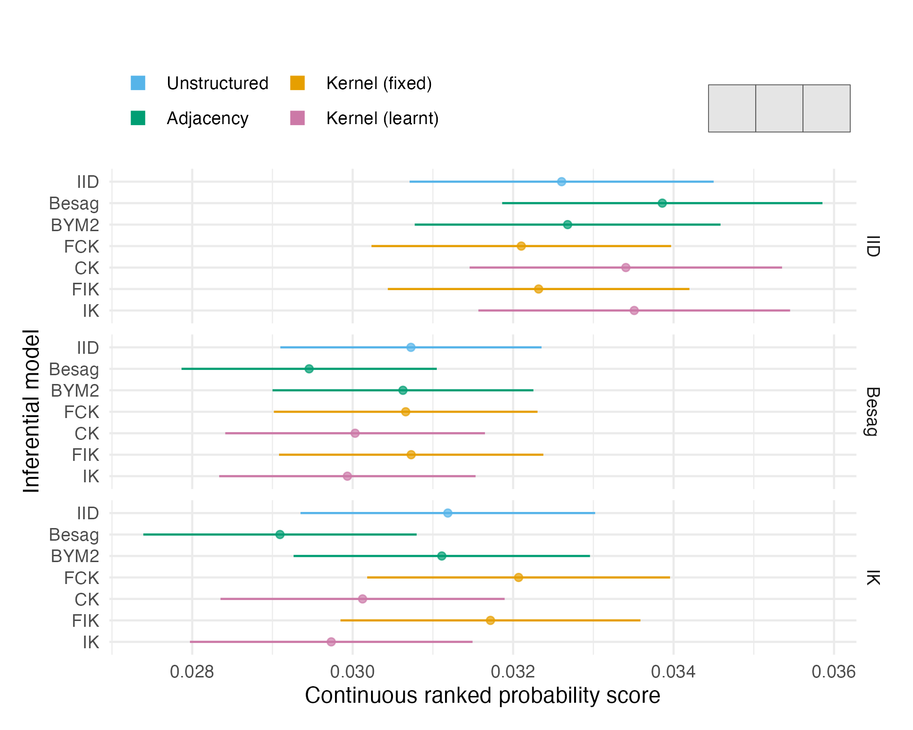
$The mean CRPS with 95% credible interval in estimating $\rho$ using each inferential model and simulation model on the first vignette geometry (Panel 4.6A). Credible intervals were generated using 1.96 times the standard error.$

Figure A.13: The mean CRPS with 95% credible interval in estimating $\rho$ using each inferential model and simulation model on the first vignette geometry (Panel 4.6A). Credible intervals were generated using 1.96 times the standard error.

$The mean CRPS with 95% credible interval in estimating $\rho$ using each inferential model and simulation model on the second vignette geometry (Panel 4.6B). Credible intervals were generated using 1.96 times the standard error.$

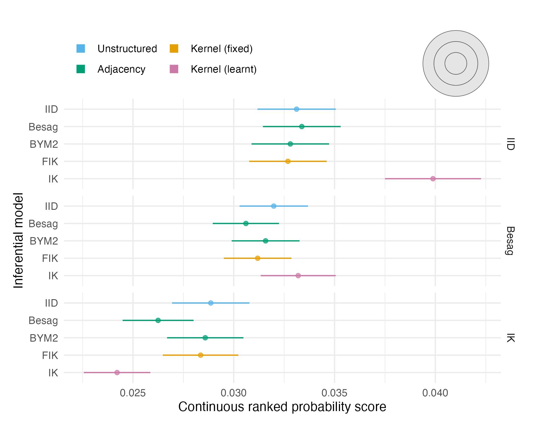
Figure A.14: The mean CRPS with 95% credible interval in estimating $\rho$ using each inferential model and simulation model on the second vignette geometry (Panel 4.6B). Credible intervals were generated using 1.96 times the standard error.

$The mean CRPS with 95% credible interval in estimating $\rho$ using each inferential model and simulation model on third vignette geometry (Panel 4.6C). Credible intervals were generated using 1.96 times the standard error.$

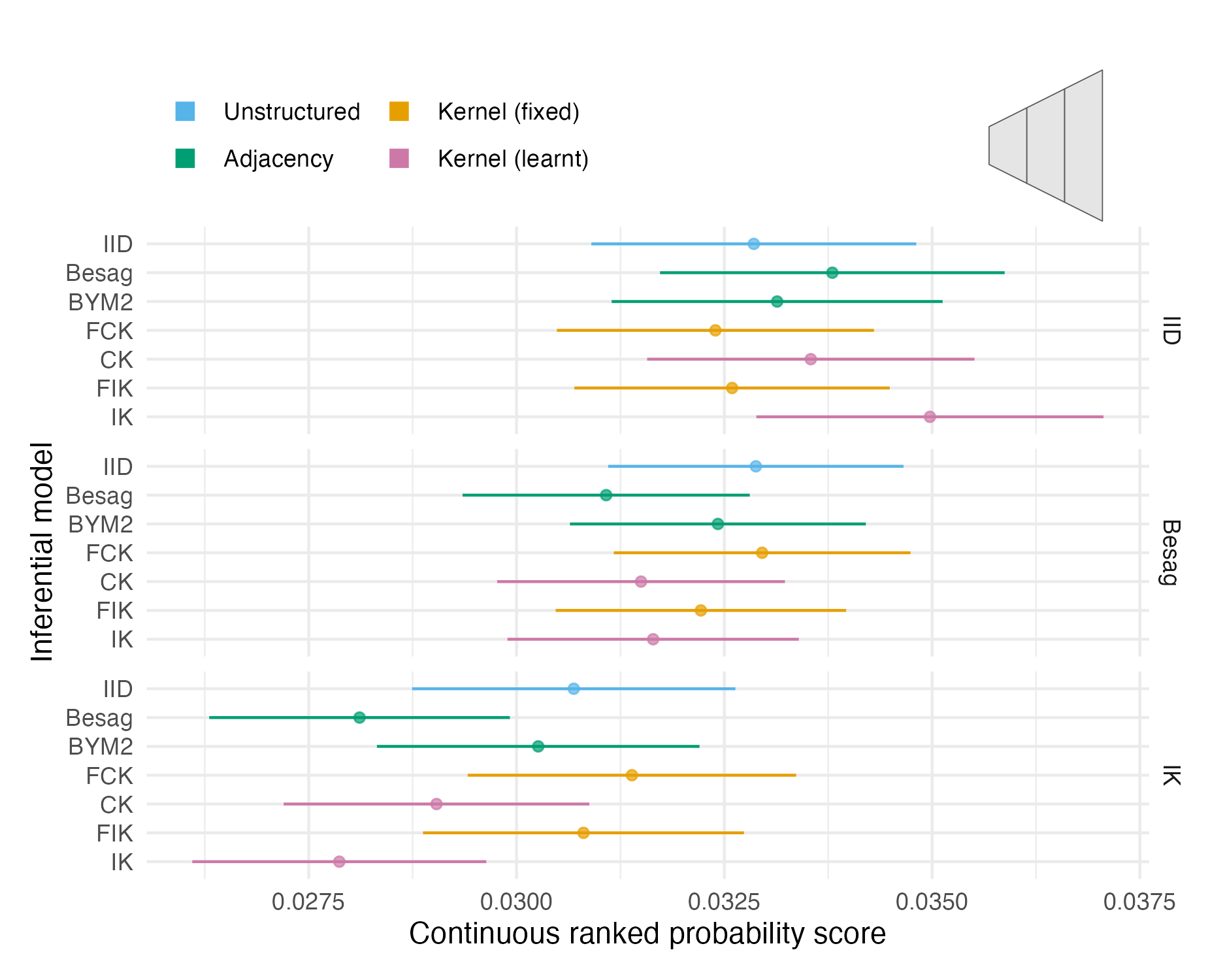
Figure A.15: The mean CRPS with 95% credible interval in estimating $\rho$ using each inferential model and simulation model on third vignette geometry (Panel 4.6C). Credible intervals were generated using 1.96 times the standard error.

$The mean CRPS with 95% credible interval in estimating $\rho$ using each inferential model and simulation model on the fourth vignette geometry (Panel 4.6D). Credible intervals were generated using 1.96 times the standard error.$

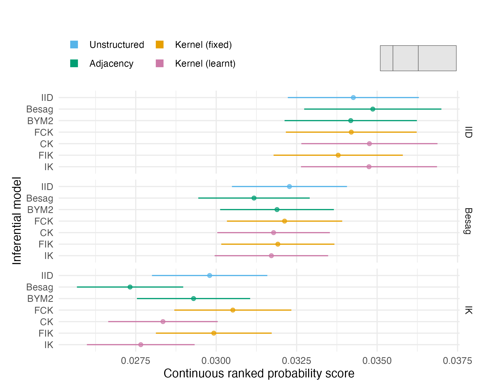
Figure A.16: The mean CRPS with 95% credible interval in estimating $\rho$ using each inferential model and simulation model on the fourth vignette geometry (Panel 4.6D). Credible intervals were generated using 1.96 times the standard error.

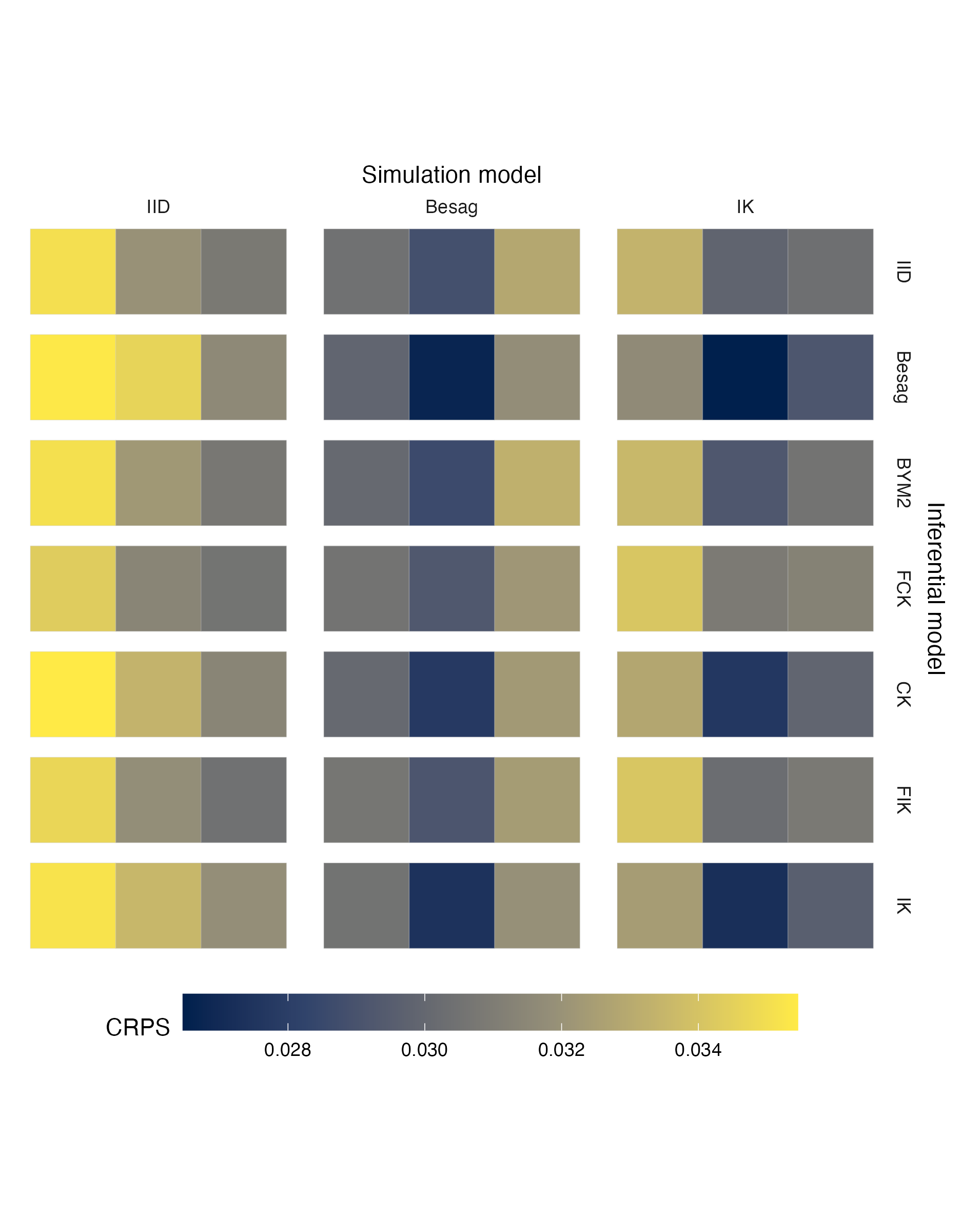
$Choropleths showing the mean value of the CRPS in estimating $\rho$, under each inferential model and simulation model, at each area of the first vignette geometry (Panel 4.6A).$

Figure A.17: Choropleths showing the mean value of the CRPS in estimating $\rho$, under each inferential model and simulation model, at each area of the first vignette geometry (Panel 4.6A).

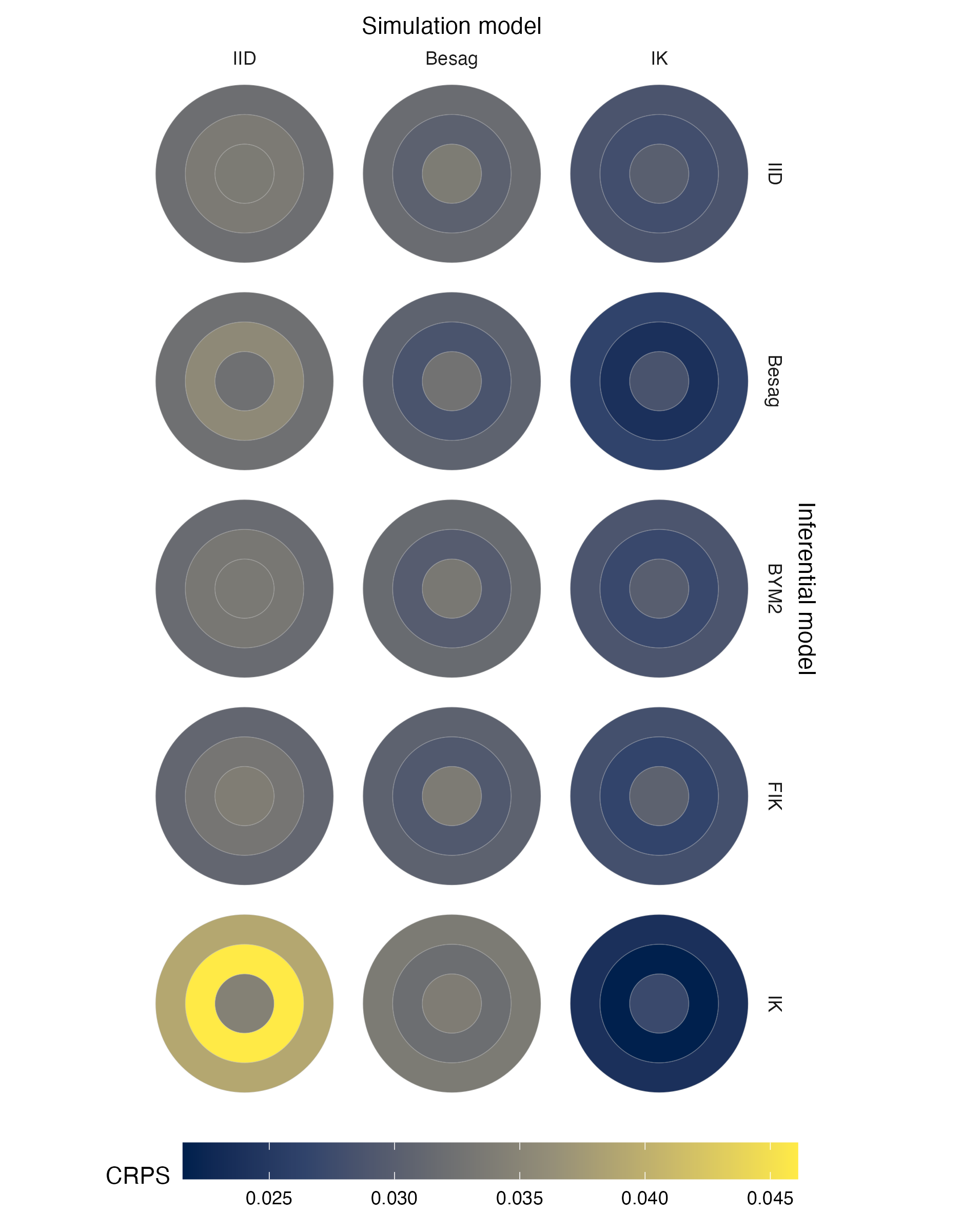
$Choropleths showing the mean value of the CRPS in estimating $\rho$, under each inferential model and simulation model, at each area of the second vignette geometry (Panel 4.6B).$

Figure A.18: Choropleths showing the mean value of the CRPS in estimating $\rho$, under each inferential model and simulation model, at each area of the second vignette geometry (Panel 4.6B).

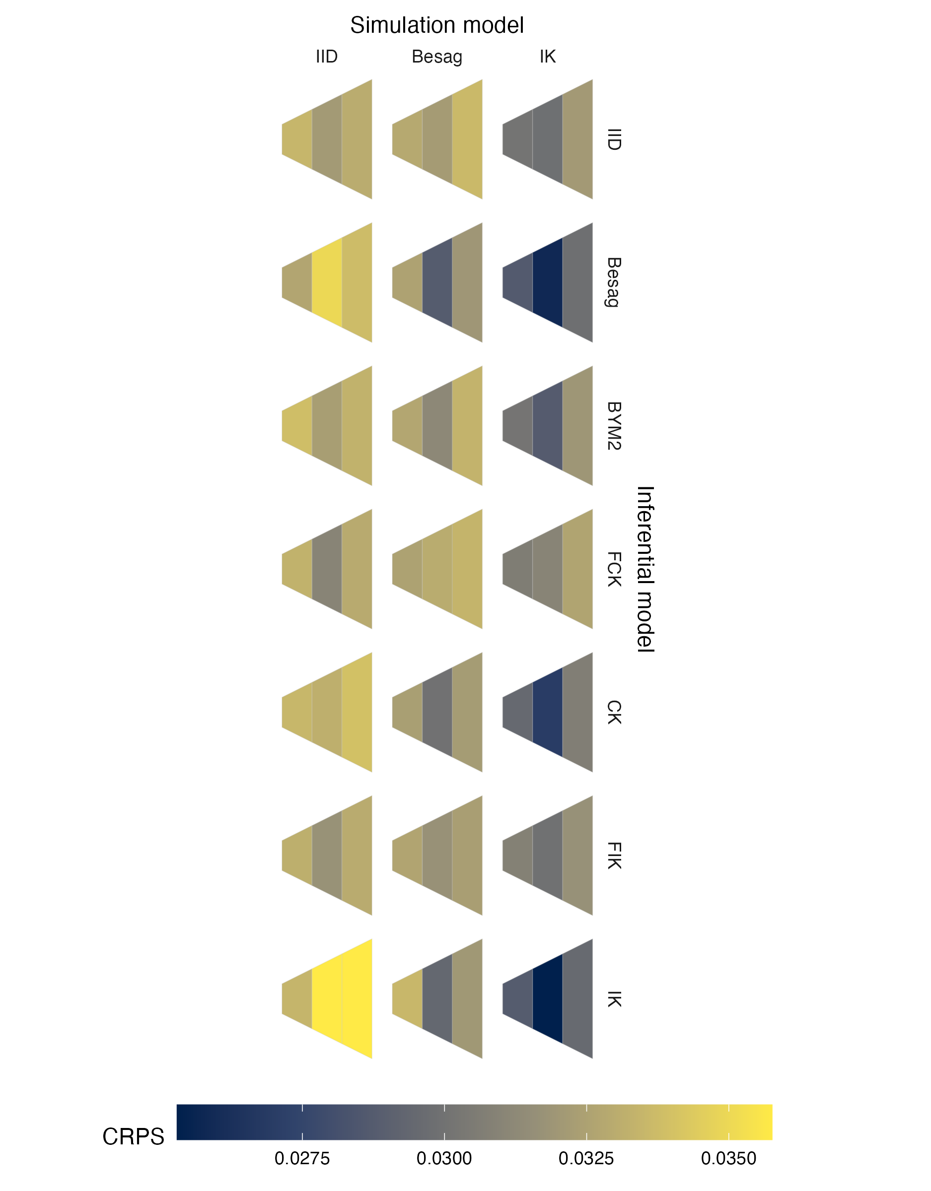
$Choropleths showing the mean value of the CRPS in estimating $\rho$, under each inferential model and simulation model, at each area of the third vignette geometry (Panel 4.6C).$

Figure A.19: Choropleths showing the mean value of the CRPS in estimating $\rho$, under each inferential model and simulation model, at each area of the third vignette geometry (Panel 4.6C).

$Choropleths showing the mean value of the CRPS in estimating $\rho$, under each inferential model and simulation model, at each area of the fourth vignette geometry (Panel 4.6D).$

Figure A.20: Choropleths showing the mean value of the CRPS in estimating $\rho$, under each inferential model and simulation model, at each area of the fourth vignette geometry (Panel 4.6D).

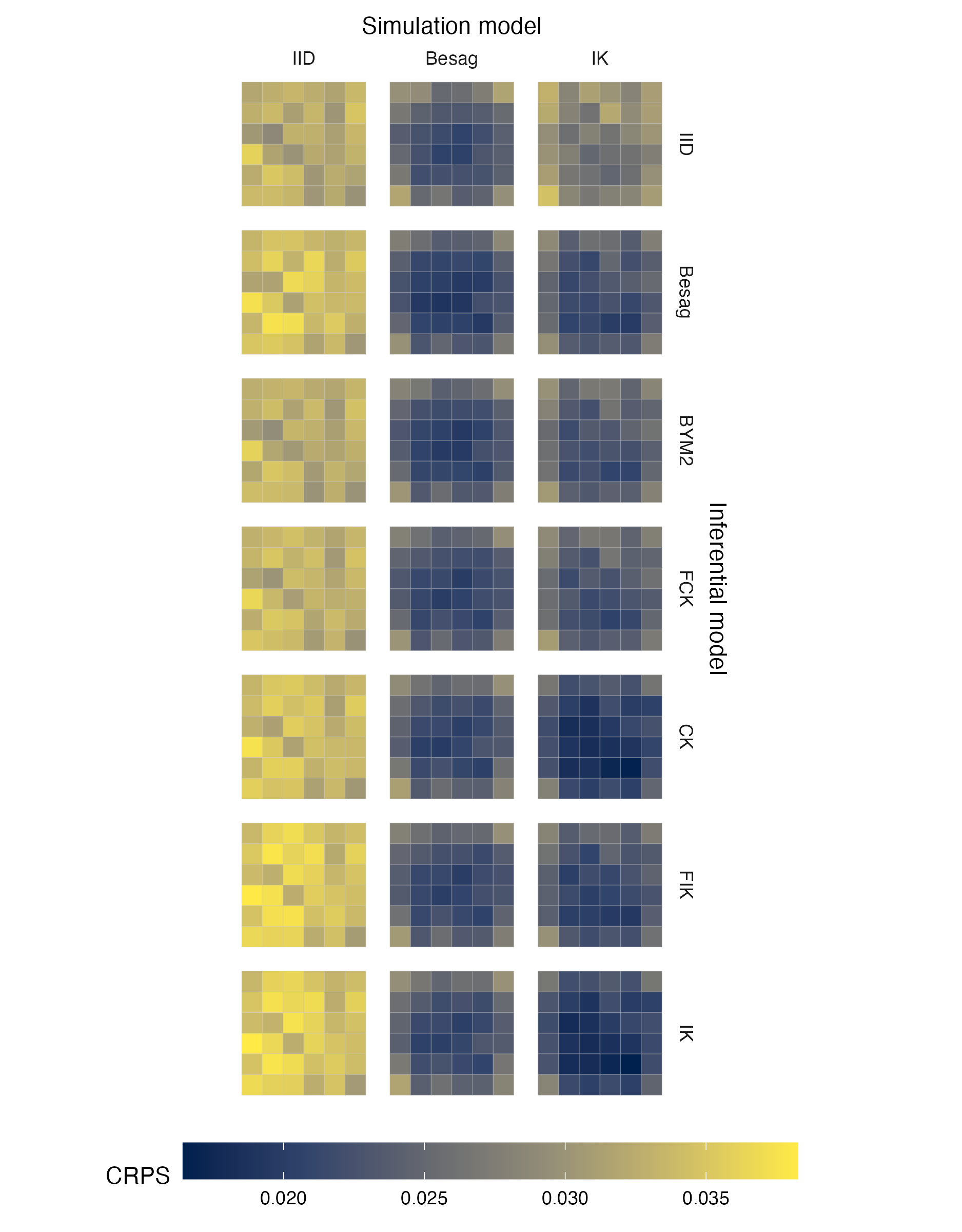
$Choropleths showing the mean value of the CRPS in estimating $\rho$, under each inferential model and simulation model, at each area of the grid geometry (Panel 4.6E).$

Figure A.21: Choropleths showing the mean value of the CRPS in estimating $\rho$, under each inferential model and simulation model, at each area of the grid geometry (Panel 4.6E).

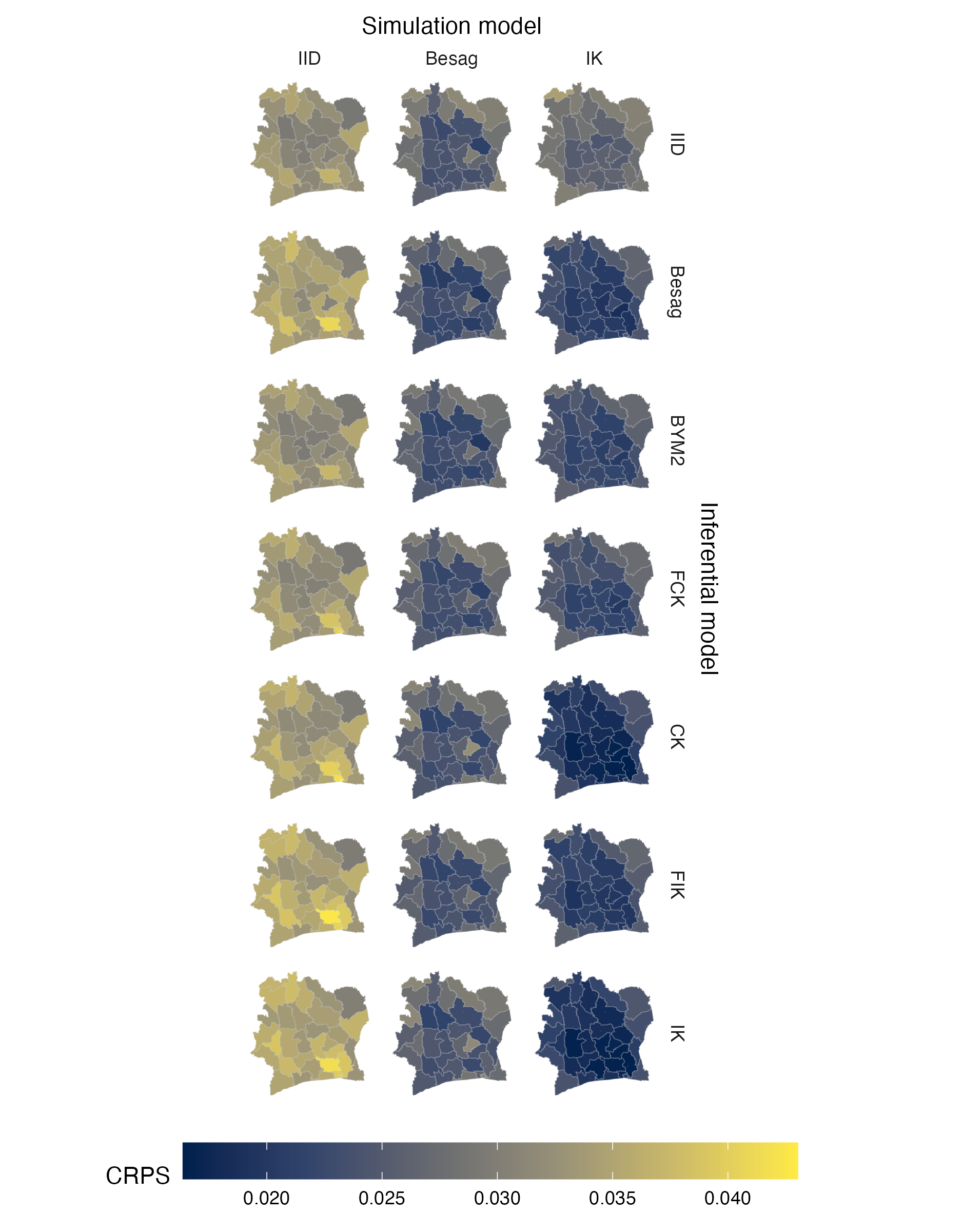
$Choropleths showing the mean value of the CRPS in estimating $\rho$, under each inferential model and simulation model, at each area of the Côte d’Ivoire geometry (Panel 4.6F).$

Figure A.22: Choropleths showing the mean value of the CRPS in estimating $\rho$, under each inferential model and simulation model, at each area of the Côte d’Ivoire geometry (Panel 4.6F).

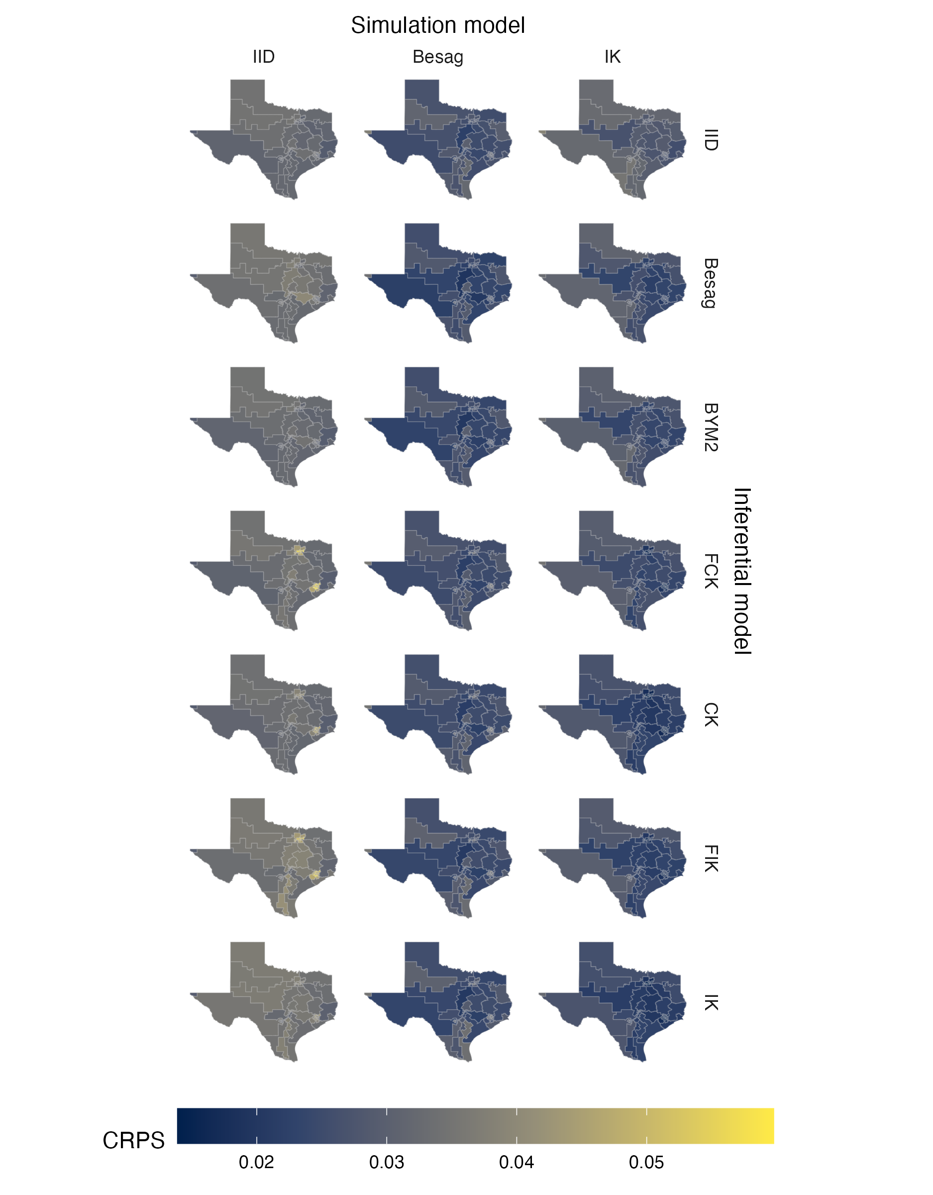
$Choropleths showing the mean value of the CRPS in estimating $\rho$, under each inferential model and simulation model, at each area of the Texas geometry (Panel 4.6G).$

Figure A.23: Choropleths showing the mean value of the CRPS in estimating $\rho$, under each inferential model and simulation model, at each area of the Texas geometry (Panel 4.6G).

A.3.5 Calibration

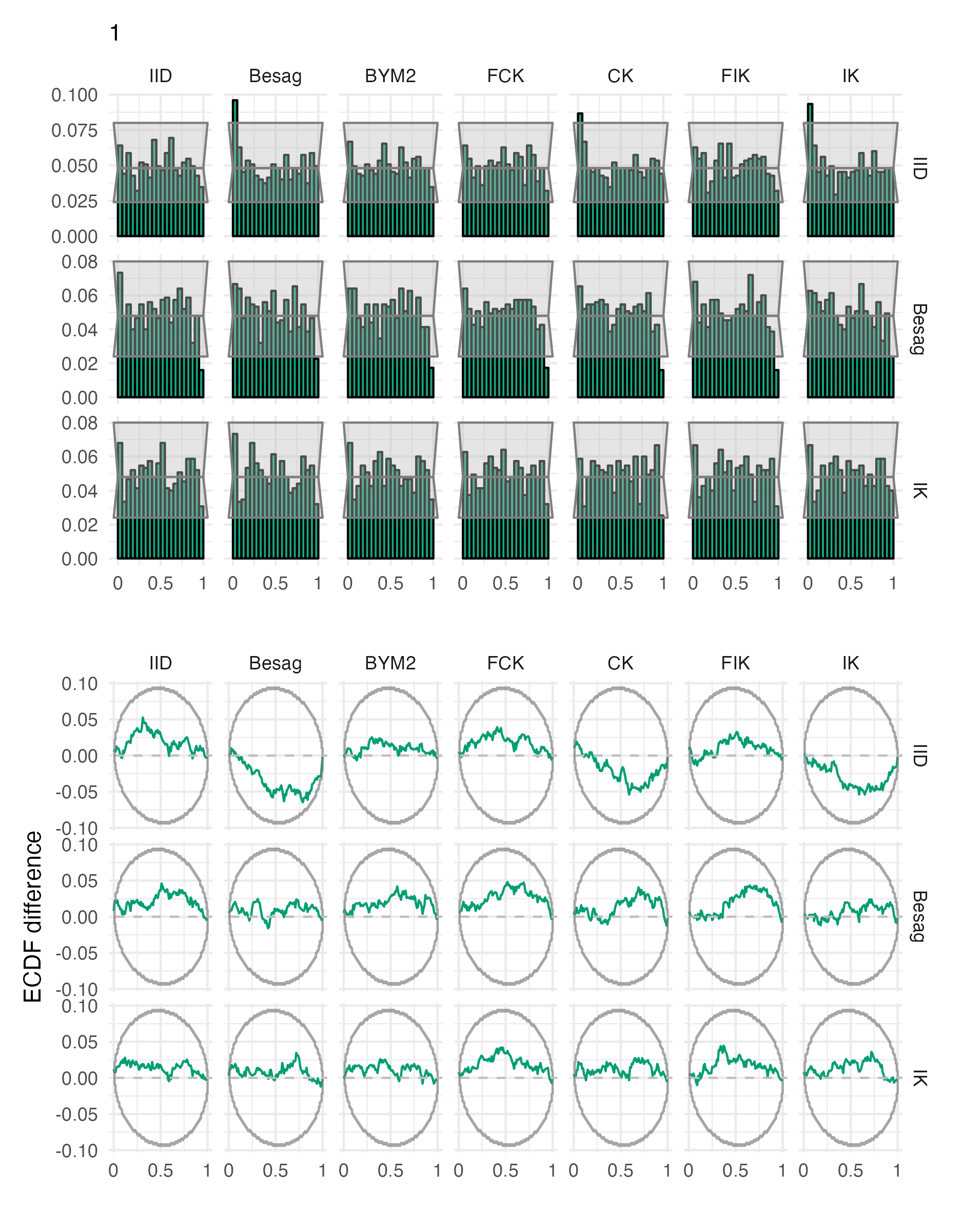
$Probability integral transform histograms and empirical cumulative distribution function difference plots for $\rho$, under each inferential model and simulation model, for the first vignette geometry (Panel 4.6A).$

Figure A.24: Probability integral transform histograms and empirical cumulative distribution function difference plots for $\rho$, under each inferential model and simulation model, for the first vignette geometry (Panel 4.6A).

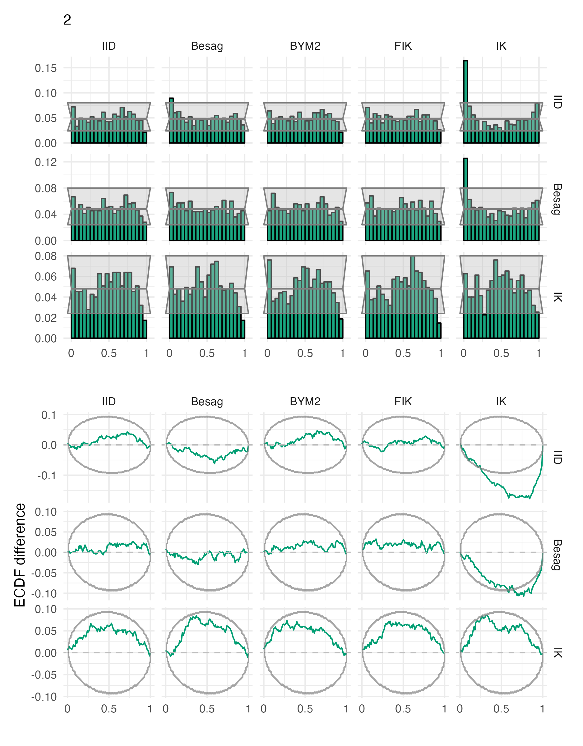
Figure A.25: Probability integral transform histograms and empirical cumulative distribution function difference plots for $\rho$, under each inferential model and simulation model, for the second vignette geometry (Panel 4.6B).

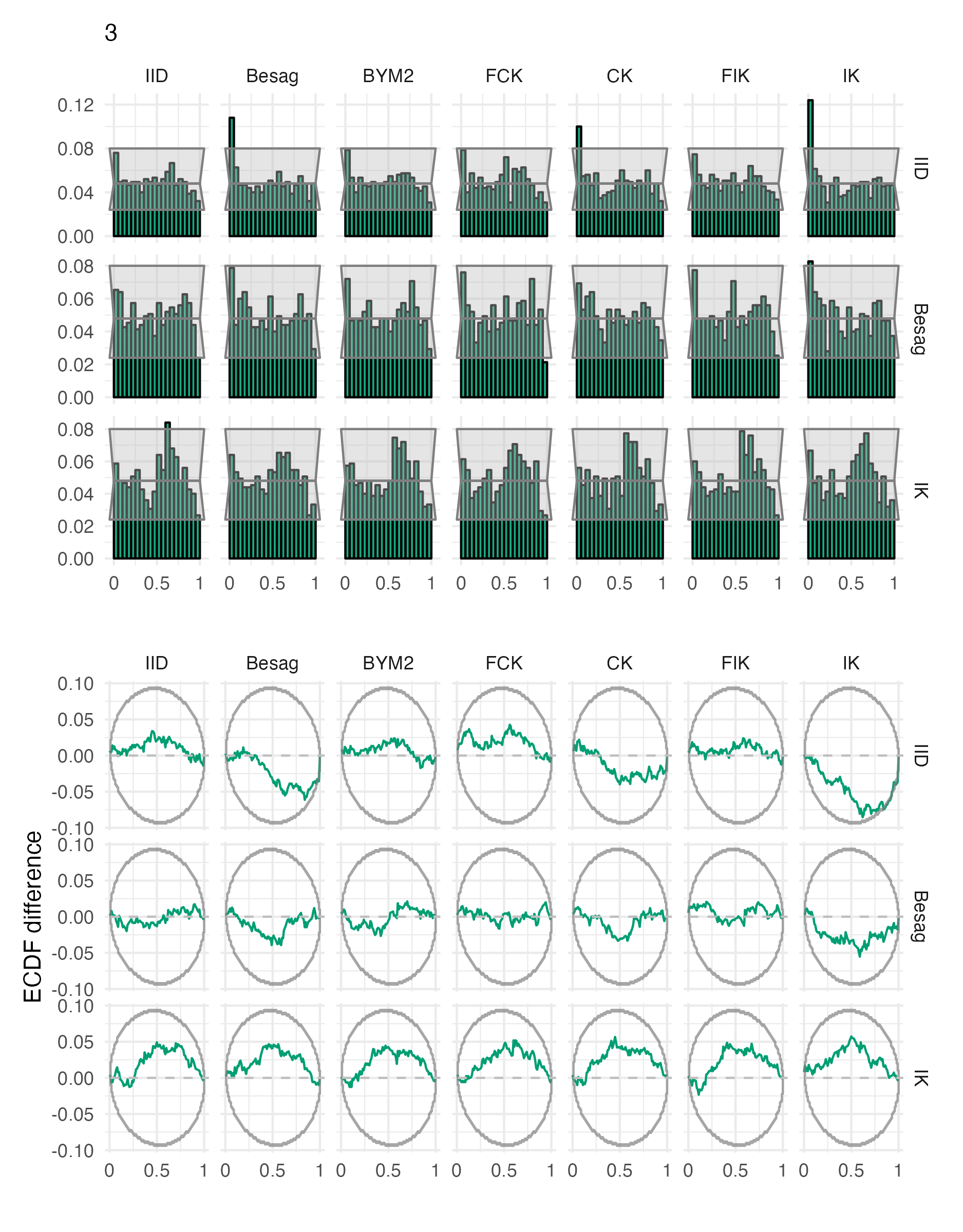
Figure A.26: Probability integral transform histograms and empirical cumulative distribution function difference plots for $\rho$, under each inferential model and simulation model, for the third vignette geometry (Panel 4.6C).

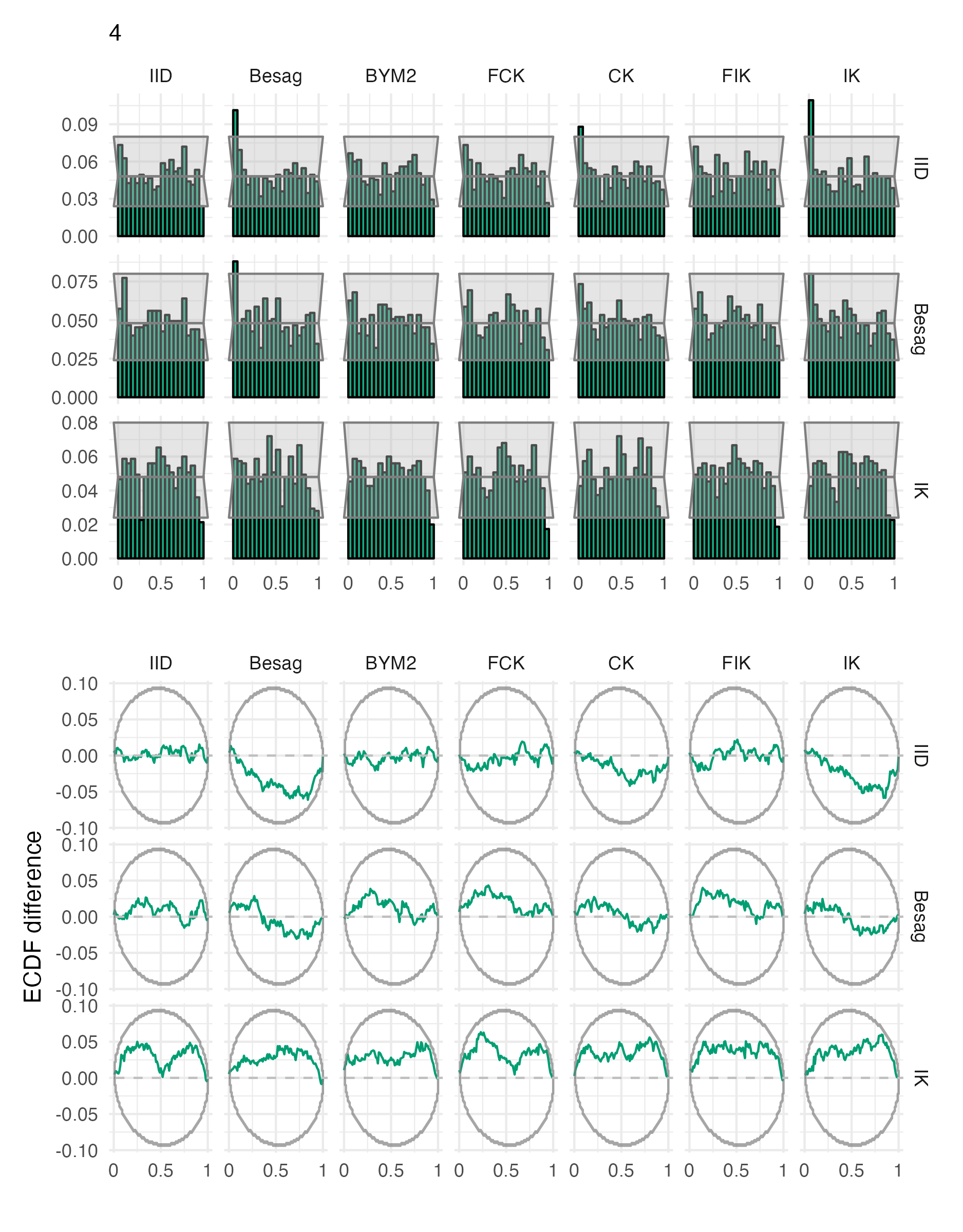
Figure A.27: Probability integral transform histograms and empirical cumulative distribution function difference plots for $\rho$, under each inferential model and simulation model, for the fourth vignette geometry (Panel 4.6D).

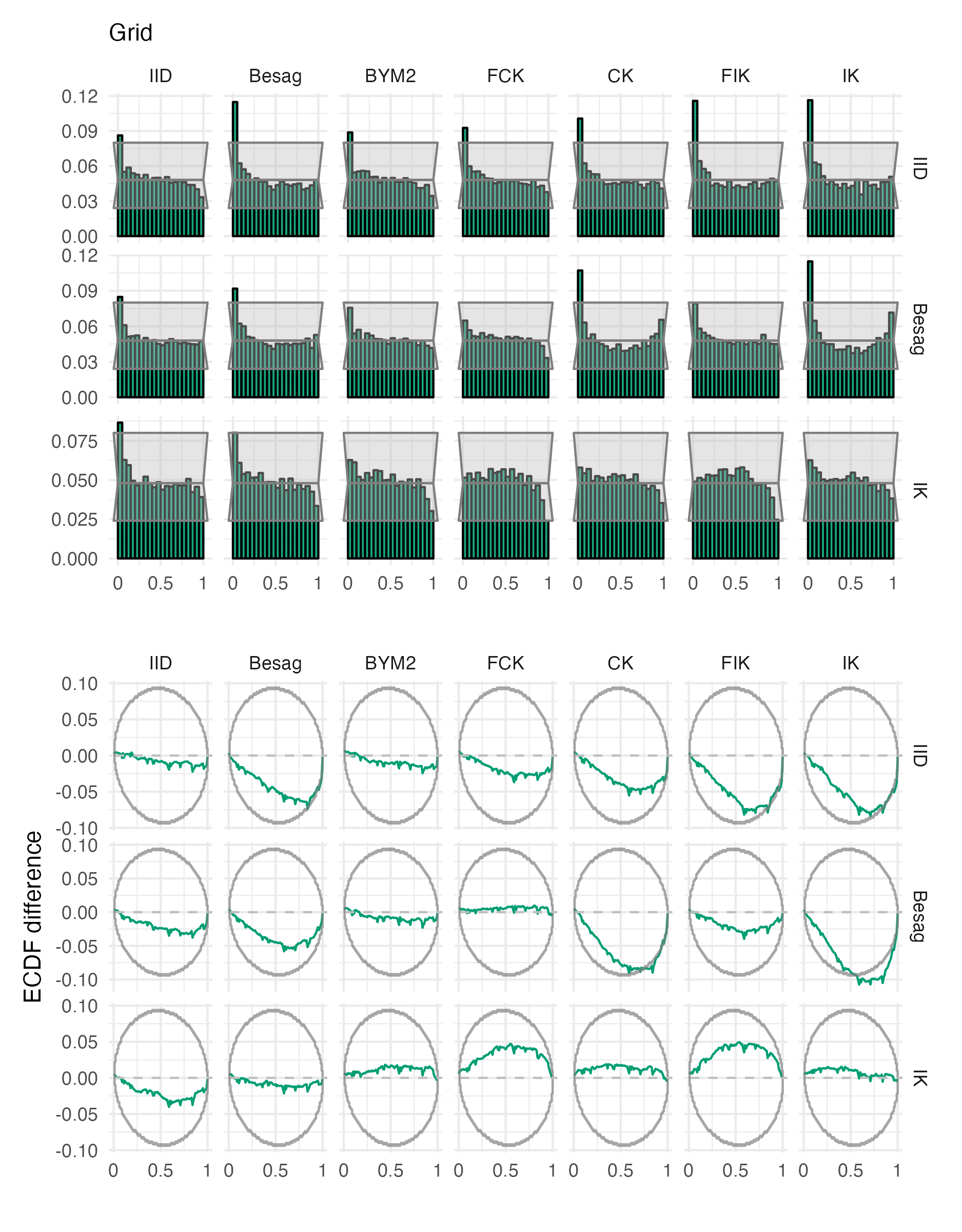
Figure A.28: Probability integral transform histograms and empirical cumulative distribution function difference plots for $\rho$, under each inferential model and simulation model, for the grid geometry (Panel 4.6E).

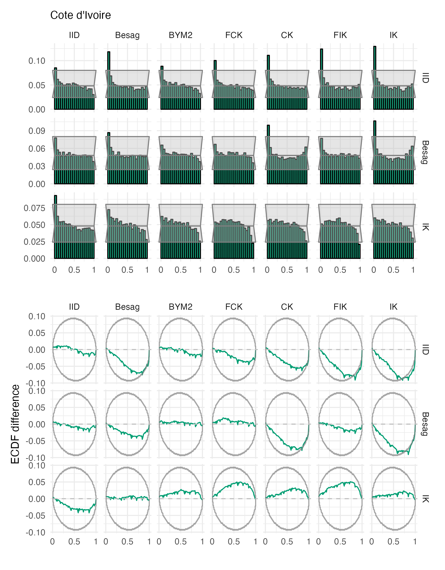
Figure A.29: Probability integral transform histograms and empirical cumulative distribution function difference plots for $\rho$, under each inferential model and simulation model, for the Côte d’Ivoire geometry (Panel 4.6F).

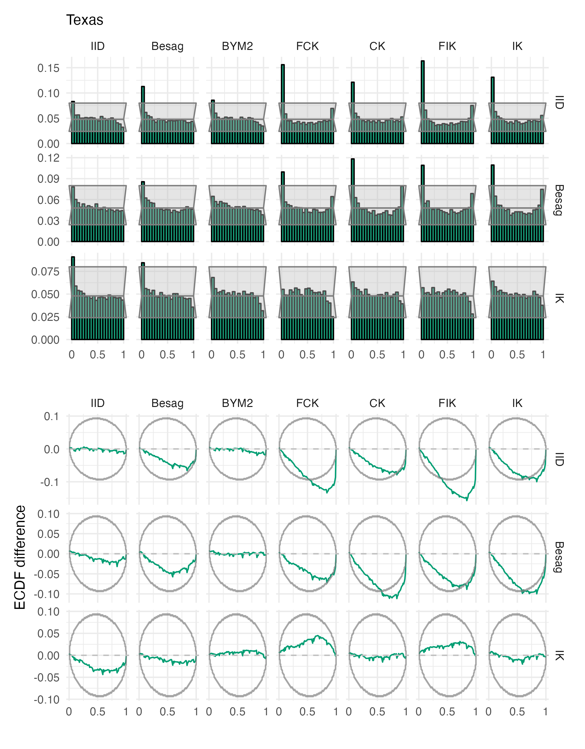
Figure A.30: Probability integral transform histograms and empirical cumulative distribution function difference plots for $\rho$, under each inferential model and simulation model, for the Texas geometry (Panel 4.6G).

A.4 HIV study

A.4.1 Lengthscale

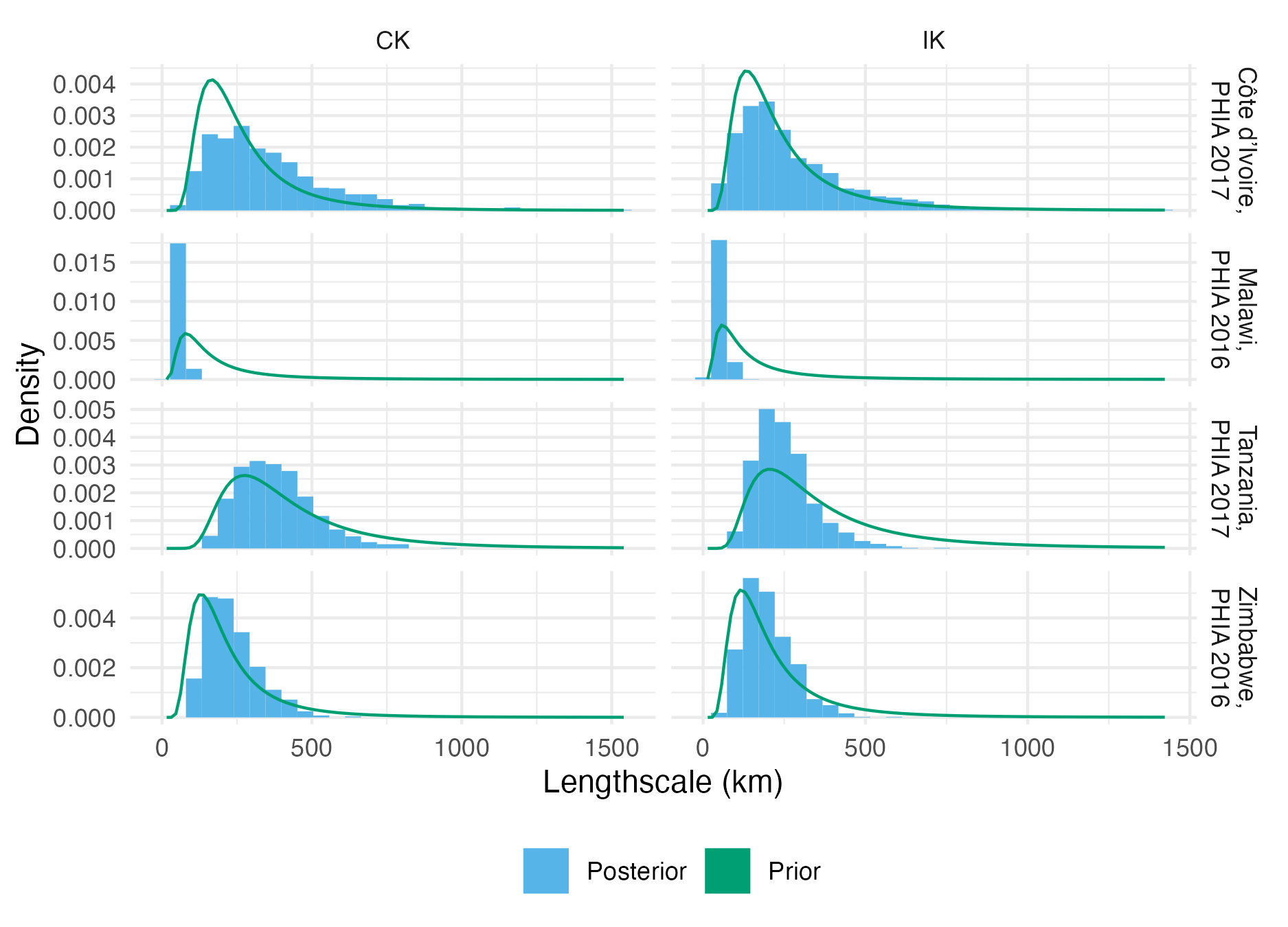
The lengthscale hyperparameter prior and posterior distributions for each of the four considered PHIA surveys (Table 4.3), using both the CK and IK inferential models.

Figure A.31: The lengthscale hyperparameter prior and posterior distributions for each of the four considered PHIA surveys (Table 4.3), using both the CK and IK inferential models.

A.4.2 BYM2 proportion

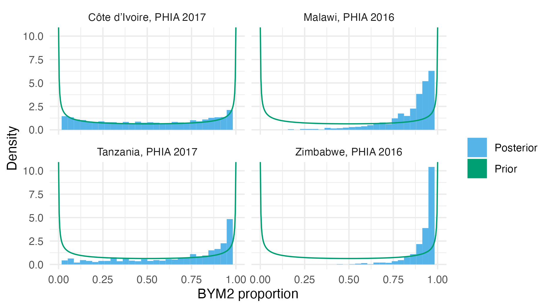
The BYM2 proportion hyperparameter prior and posterior distributions for each of the four considered PHIA surveys (Table 4.3). A value of zero corresponds to IID noise. A value of one corresponds to Besag noise. For each survey, excluding the Côte d’Ivoire 2017 PHIA, the posterior distribution for the BYM2 proportion is concentrated towards a value of one. This result can be interpreted as suggesting that the variation in HIV prevalence from these surveys is spatially structured.

Figure A.32: The BYM2 proportion hyperparameter prior and posterior distributions for each of the four considered PHIA surveys (Table 4.3). A value of zero corresponds to IID noise. A value of one corresponds to Besag noise. For each survey, excluding the Côte d’Ivoire 2017 PHIA, the posterior distribution for the BYM2 proportion is concentrated towards a value of one. This result can be interpreted as suggesting that the variation in HIV prevalence from these surveys is spatially structured.

A.4.3 Estimates

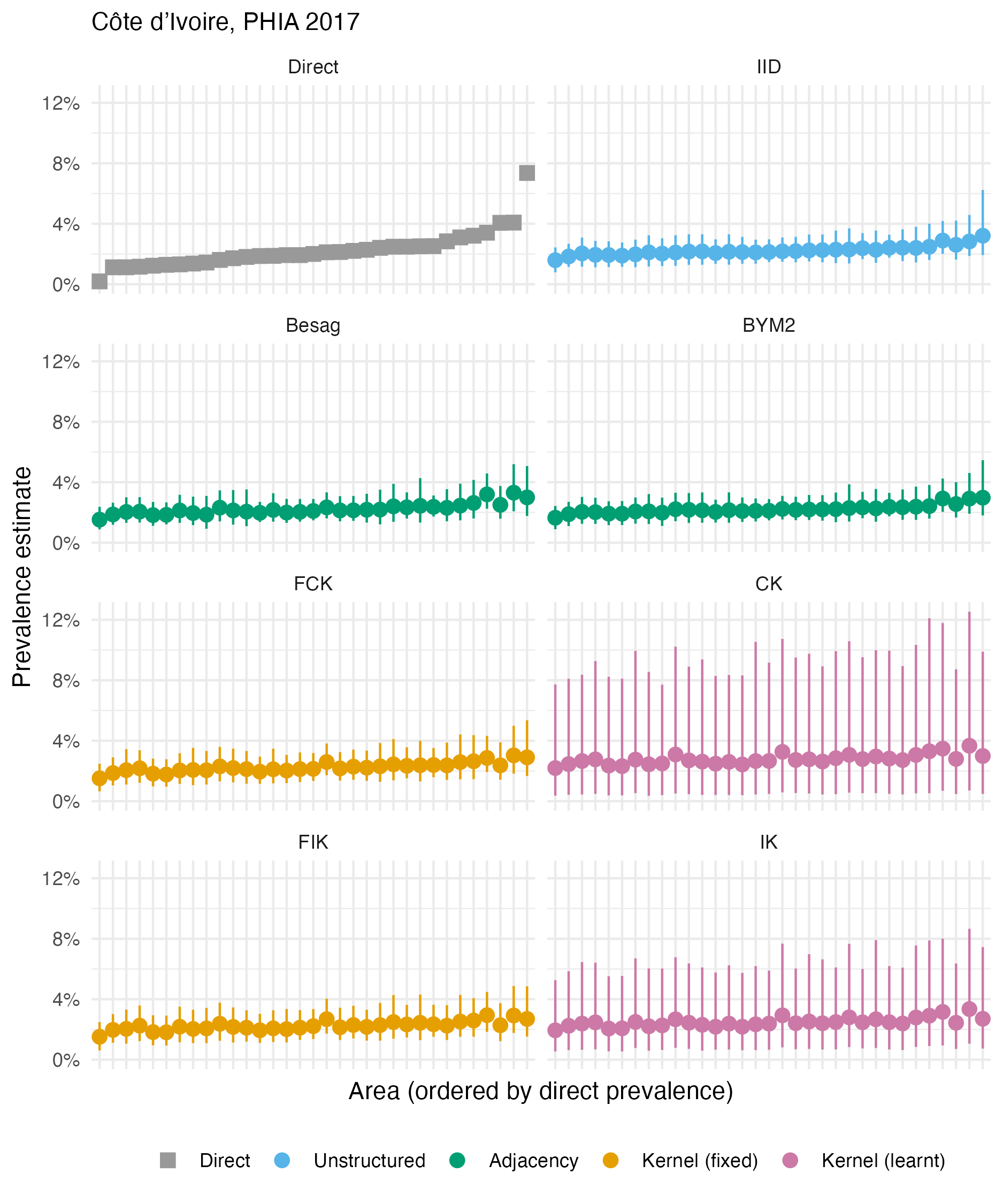
The HIV prevalence posterior mean and 95% credible interval for each area of Côte d’Ivoire, based on the 2017 PHIA survey. Direct estimates obtained from the survey are as shown in Panel 4.10A.

Figure A.33: The HIV prevalence posterior mean and 95% credible interval for each area of Côte d’Ivoire, based on the 2017 PHIA survey. Direct estimates obtained from the survey are as shown in Panel 4.10A.

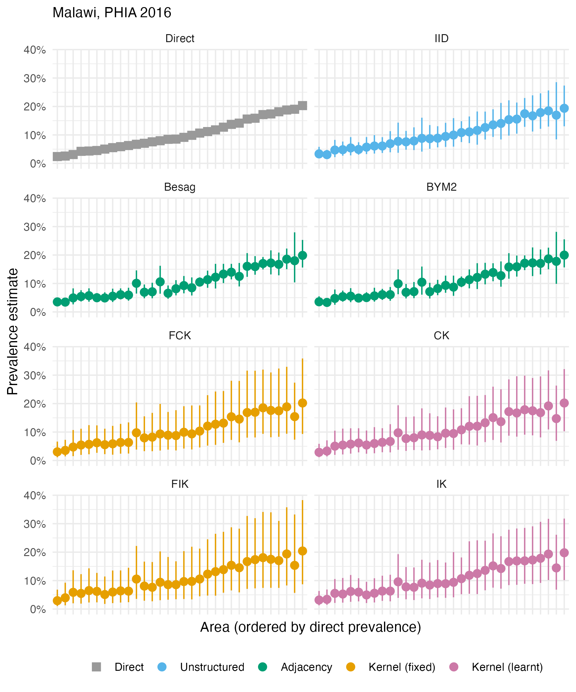
The HIV prevalence posterior mean and 95% credible interval for each area of Malawi, based on the 2016 PHIA survey. Direct estimates obtained from the survey are as shown in Panel 4.10B.

Figure A.34: The HIV prevalence posterior mean and 95% credible interval for each area of Malawi, based on the 2016 PHIA survey. Direct estimates obtained from the survey are as shown in Panel 4.10B.

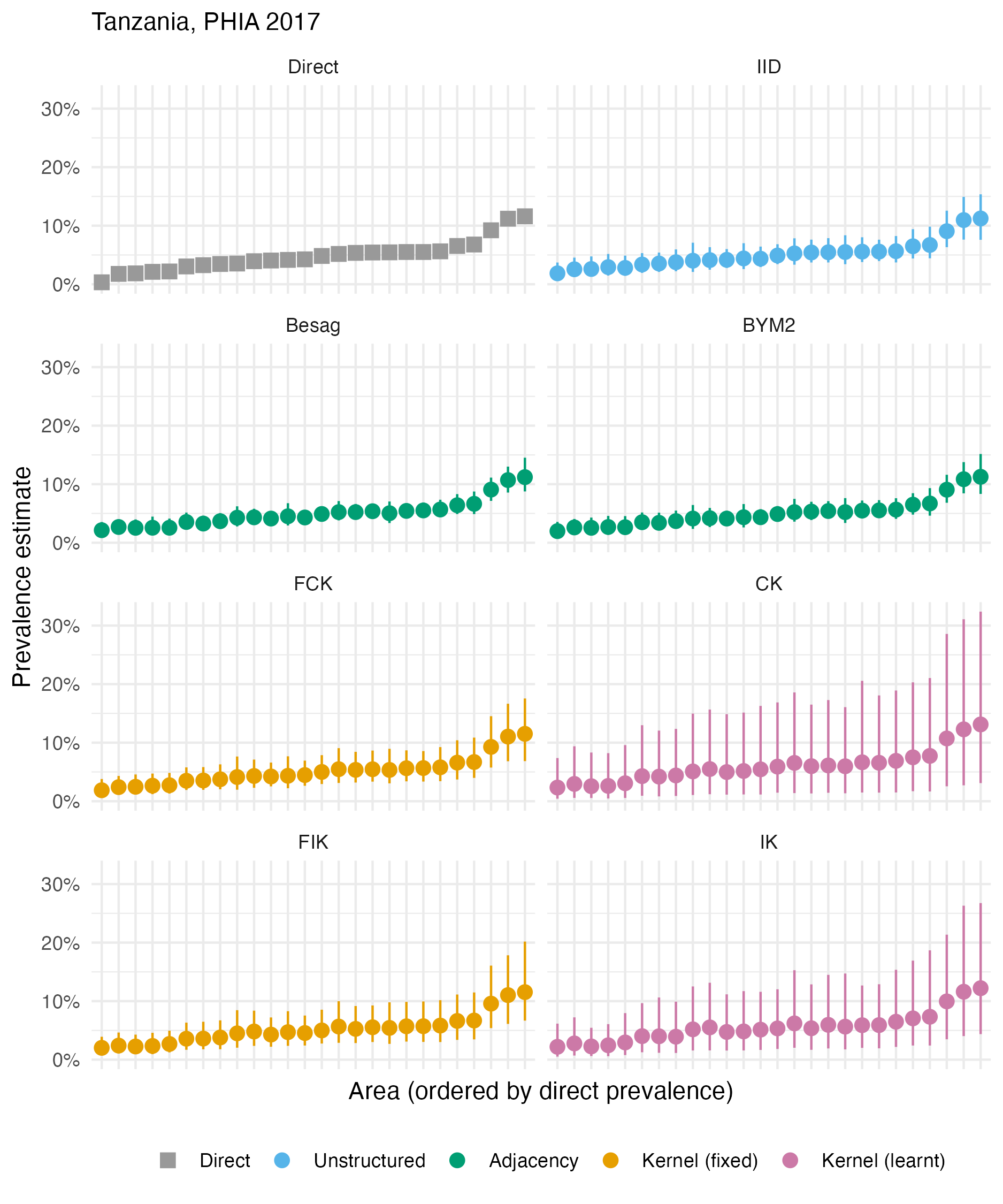
The HIV prevalence posterior mean and 95% credible interval for each area of Tanzania, based on the 2017 PHIA survey. Direct estimates obtained from the survey are as shown in Panel 4.10C.

Figure A.35: The HIV prevalence posterior mean and 95% credible interval for each area of Tanzania, based on the 2017 PHIA survey. Direct estimates obtained from the survey are as shown in Panel 4.10C.

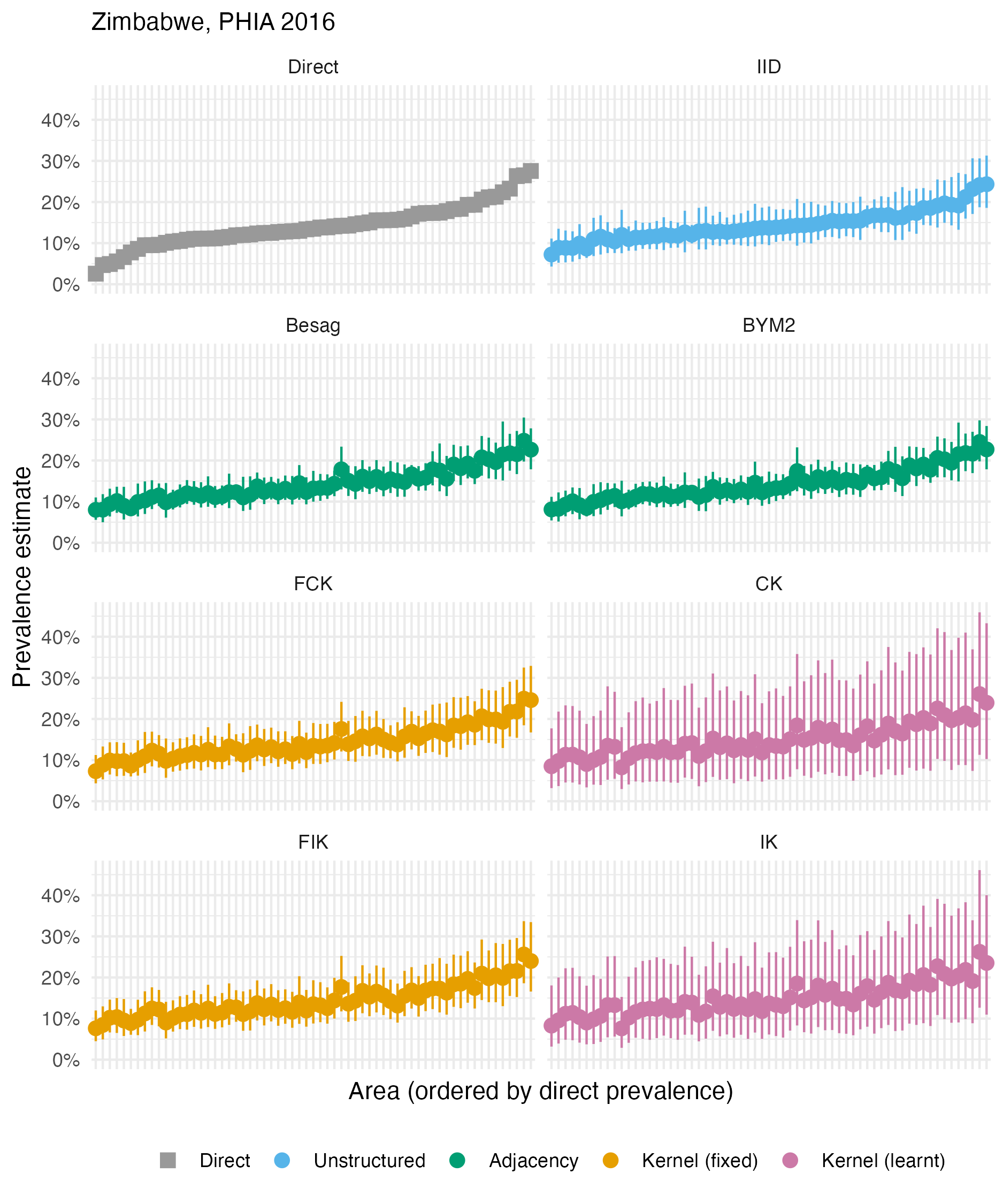
The HIV prevalence posterior mean and 95% credible interval for each area of Zimbabwe, based on the 2016 PHIA survey. Direct estimates obtained from the survey are as shown in Panel 4.10D.

Figure A.36: The HIV prevalence posterior mean and 95% credible interval for each area of Zimbabwe, based on the 2016 PHIA survey. Direct estimates obtained from the survey are as shown in Panel 4.10D.

A.4.4 Cross-validation

A.4.4.1 Mean squared error

Table A.4: The mean pointwise leave-one-out and spatial leave-one-out MSE in estimating $\rho_i$, with standard errors, for each inferential model across the four considered PHIA surveys. The units used in this table are thousandths.
PHIA survey	Mean squared error (units: 1/1000)
PHIA survey	IID	Besag	BYM2	FCK	CK	FIK	IK
LOO
Côte d’Ivoire, 2017	0.21	0.22	0.20	0.21	0.19	0.21	0.20
Malawi, 2016	7.10	2.39	2.59	3.59	3.70	2.43	2.54
Tanzania, 2017	1.66	1.14	1.43	0.95	0.65	0.78	0.66
Zimbabwe, 2016	4.76	2.51	2.54	2.51	1.88	2.15	1.83
SLOO
Côte d’Ivoire, 2017	0.20	0.22	0.21	0.24	0.25	0.26	0.25
Malawi, 2016	7.13	2.41	3.32	8.22	7.95	7.05	6.70
Tanzania, 2017	1.65	1.09	2.46	1.86	2.80	1.86	2.59
Zimbabwe, 2016	4.73	2.49	3.44	3.95	3.36	3.93	3.42

A.4.4.2 Continuous ranked probability score

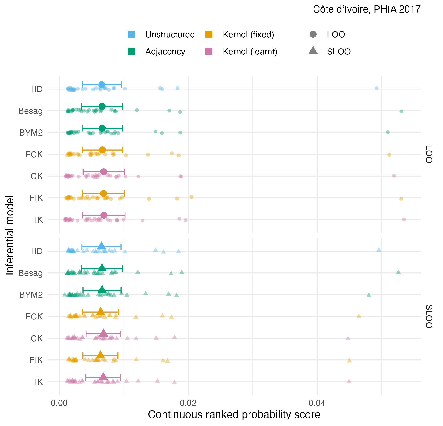
$The pointwise CRPS in estimating $\rho_i$ using either leave-one-out or spatial leave-one-out cross-validation, with mean and 95% credible interval for the Côte d’Ivoire 2017 PHIA survey (Panel 4.10A).$

Figure A.37: The pointwise CRPS in estimating $\rho_i$ using either leave-one-out or spatial leave-one-out cross-validation, with mean and 95% credible interval for the Côte d’Ivoire 2017 PHIA survey (Panel 4.10A).

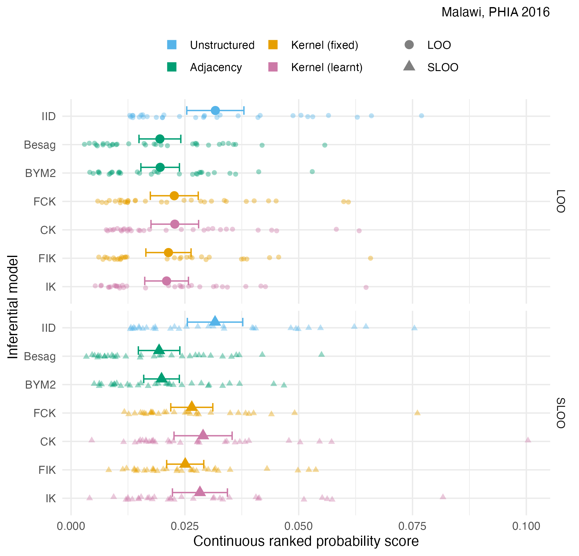
$The pointwise CRPS in estimating $\rho_i$ using either leave-one-out or spatial leave-one-out cross-validation, with mean and 95% credible interval, for the Malawi 2016 PHIA survey 4.10B.$

Figure A.38: The pointwise CRPS in estimating $\rho_i$ using either leave-one-out or spatial leave-one-out cross-validation, with mean and 95% credible interval, for the Malawi 2016 PHIA survey 4.10B.

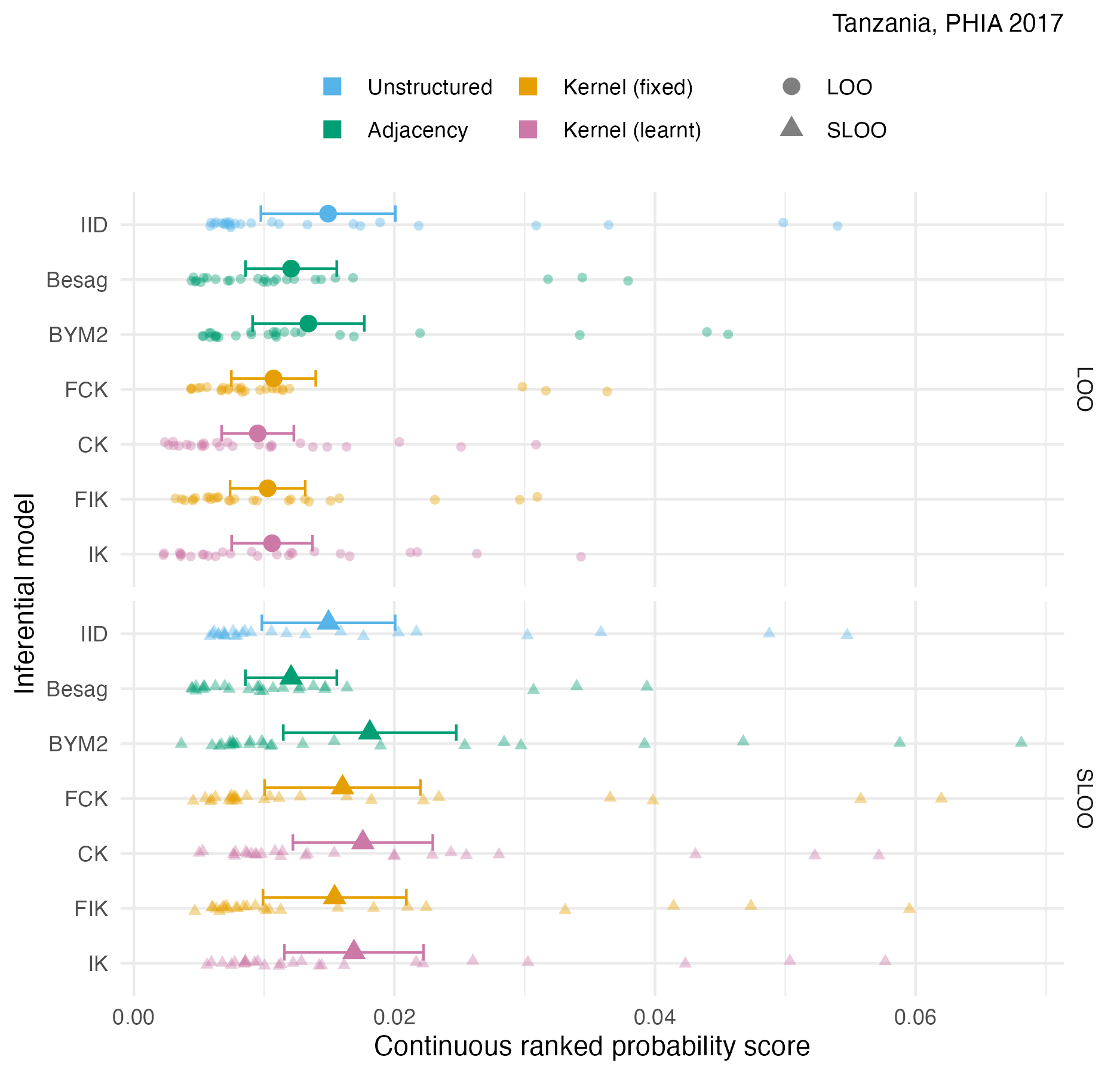
$The pointwise CRPS in estimating $\rho_i$ using either leave-one-out or spatial leave-one-out cross-validation, with mean and 95% credible interval, for the Tanzania 2017 PHIA survey 4.10C.$

Figure A.39: The pointwise CRPS in estimating $\rho_i$ using either leave-one-out or spatial leave-one-out cross-validation, with mean and 95% credible interval, for the Tanzania 2017 PHIA survey 4.10C.

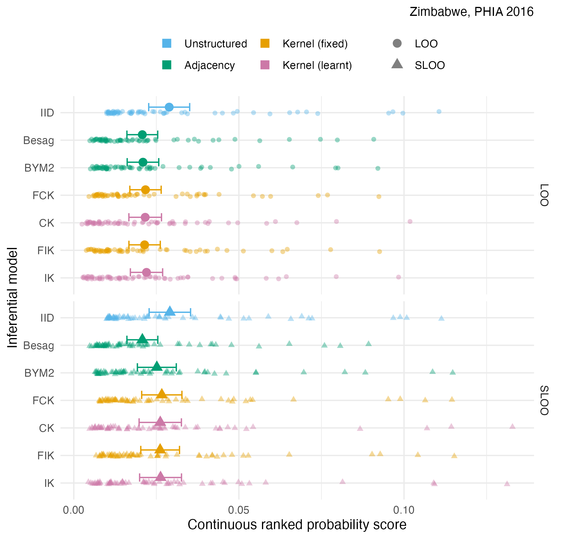
$The pointwise CRPS in estimating $\rho_i$ using either leave-one-out or spatial leave-one-out cross-validation, with mean and 95% credible interval, for the Zimbabwe 2016 PHIA survey 4.10D.$

Figure A.40: The pointwise CRPS in estimating $\rho_i$ using either leave-one-out or spatial leave-one-out cross-validation, with mean and 95% credible interval, for the Zimbabwe 2016 PHIA survey 4.10D.

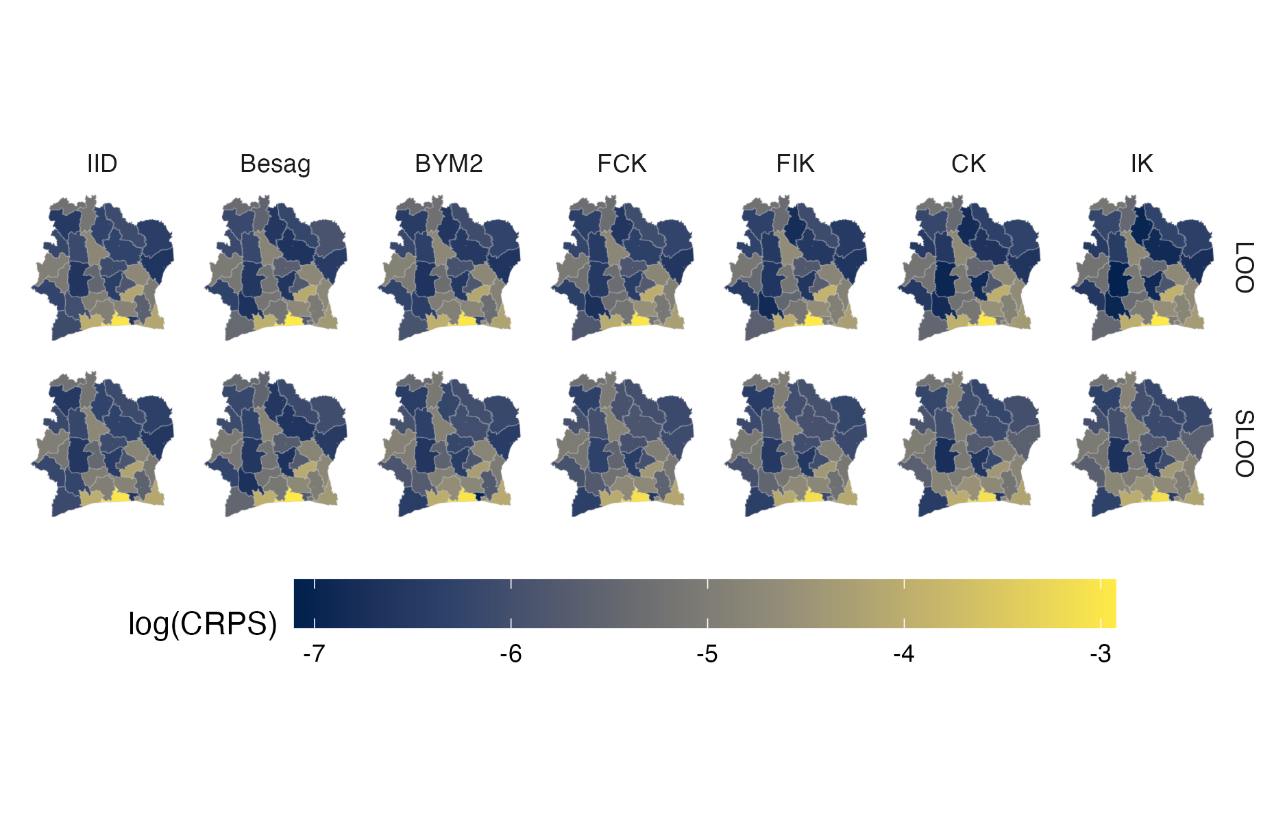
$Choropleth showing the pointwise CRPS in estimating $\rho_i$ using either leave-one-out or spatial leave-one-out cross-validation for the Côte d’Ivoire 2017 PHIA survey (Panel 4.10A).$

Figure A.41: Choropleth showing the pointwise CRPS in estimating $\rho_i$ using either leave-one-out or spatial leave-one-out cross-validation for the Côte d’Ivoire 2017 PHIA survey (Panel 4.10A).

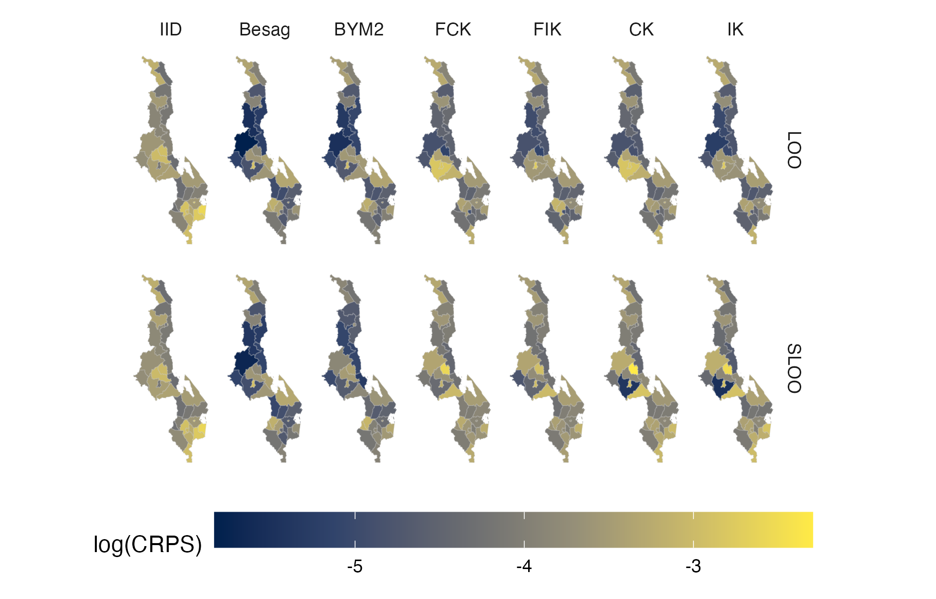
$Choropleth showing the pointwise CRPS in estimating $\rho_i$ using either leave-one-out or spatial leave-one-out cross-validation for the Malawi 2016 PHIA survey (Panel 4.10B).$

Figure A.42: Choropleth showing the pointwise CRPS in estimating $\rho_i$ using either leave-one-out or spatial leave-one-out cross-validation for the Malawi 2016 PHIA survey (Panel 4.10B).

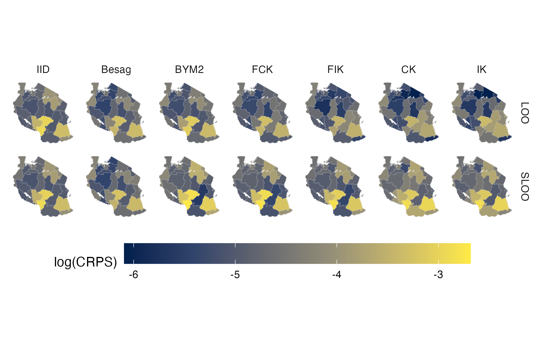
$Choropleth showing the pointwise CRPS in estimating $\rho_i$ using either leave-one-out or spatial leave-one-out cross-validation for the Tanzania 2017 PHIA survey (Panel 4.10C).$

Figure A.43: Choropleth showing the pointwise CRPS in estimating $\rho_i$ using either leave-one-out or spatial leave-one-out cross-validation for the Tanzania 2017 PHIA survey (Panel 4.10C).

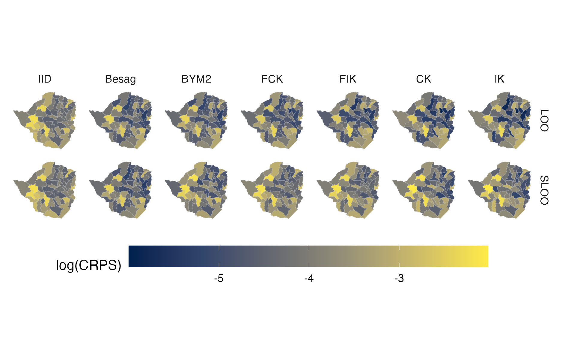
$Choropleth showing the pointwise CRPS in estimating $\rho_i$ using either leave-one-out or spatial leave-one-out cross-validation for the Zimbabwe 2016 PHIA survey (Panel 4.10D).$

Figure A.44: Choropleth showing the pointwise CRPS in estimating $\rho_i$ using either leave-one-out or spatial leave-one-out cross-validation for the Zimbabwe 2016 PHIA survey (Panel 4.10D).

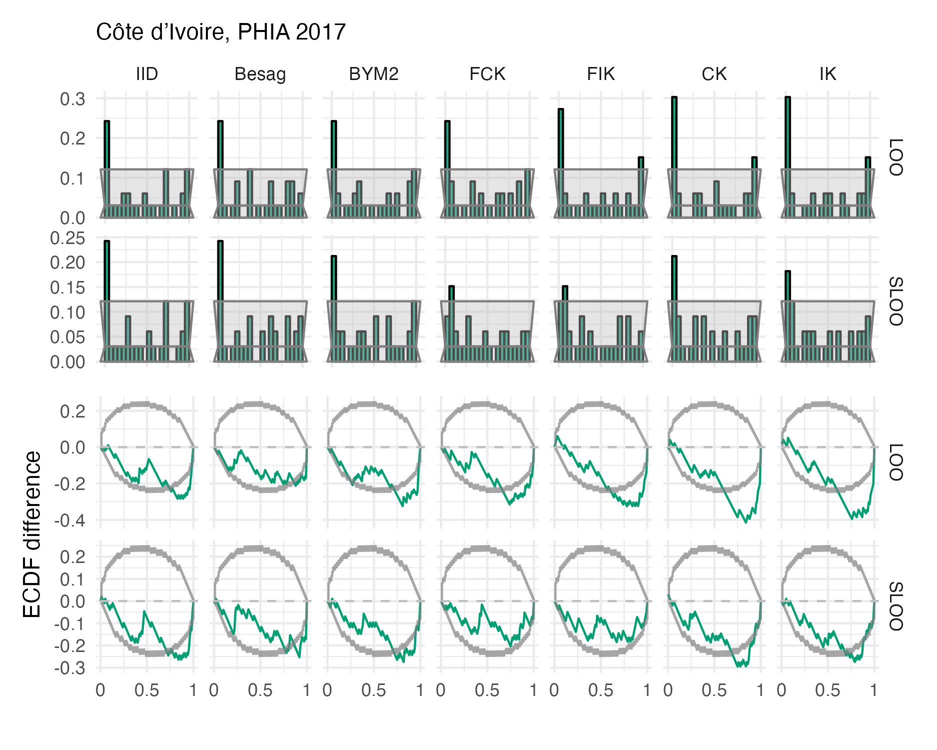
$Probability integral transform histograms and empirical cumulative distribution function difference plots in estimating $\rho$ for the Côte d’Ivoire 2017 PHIA survey (Panel 4.10A).$

Figure A.45: Probability integral transform histograms and empirical cumulative distribution function difference plots in estimating $\rho$ for the Côte d’Ivoire 2017 PHIA survey (Panel 4.10A).

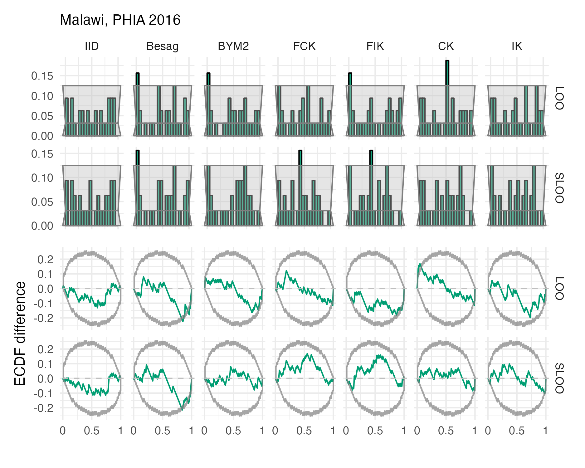
$Probability integral transform histograms and empirical cumulative distribution function difference plots in estimating $\rho$ for the Malawi 2016 PHIA survey (Panel 4.10B).$

Figure A.46: Probability integral transform histograms and empirical cumulative distribution function difference plots in estimating $\rho$ for the Malawi 2016 PHIA survey (Panel 4.10B).

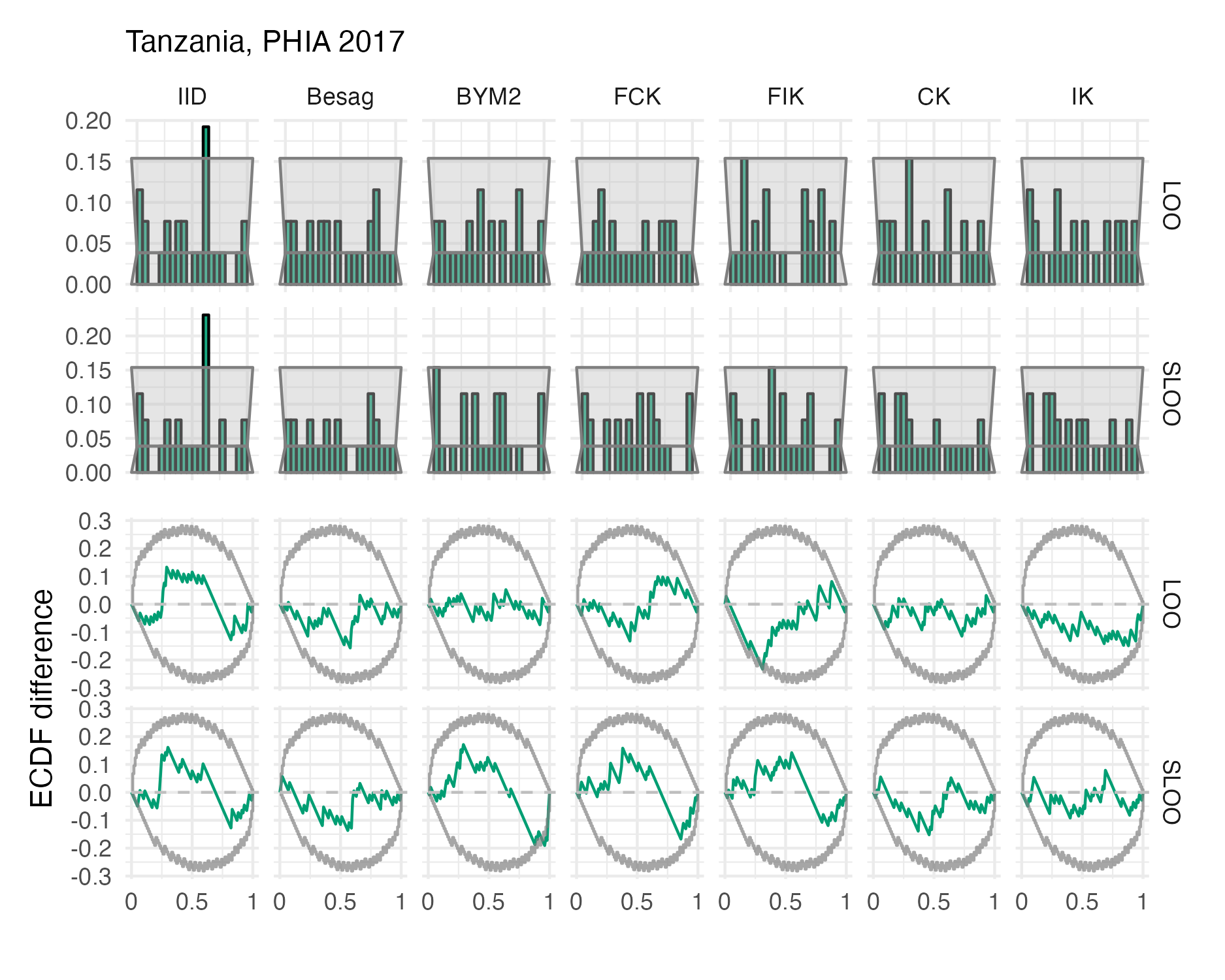
$Probability integral transform histograms and empirical cumulative distribution function difference plots in estimating $\rho$ for the Tanzania 2017 PHIA survey (Panel 4.10C).$

Figure A.47: Probability integral transform histograms and empirical cumulative distribution function difference plots in estimating $\rho$ for the Tanzania 2017 PHIA survey (Panel 4.10C).

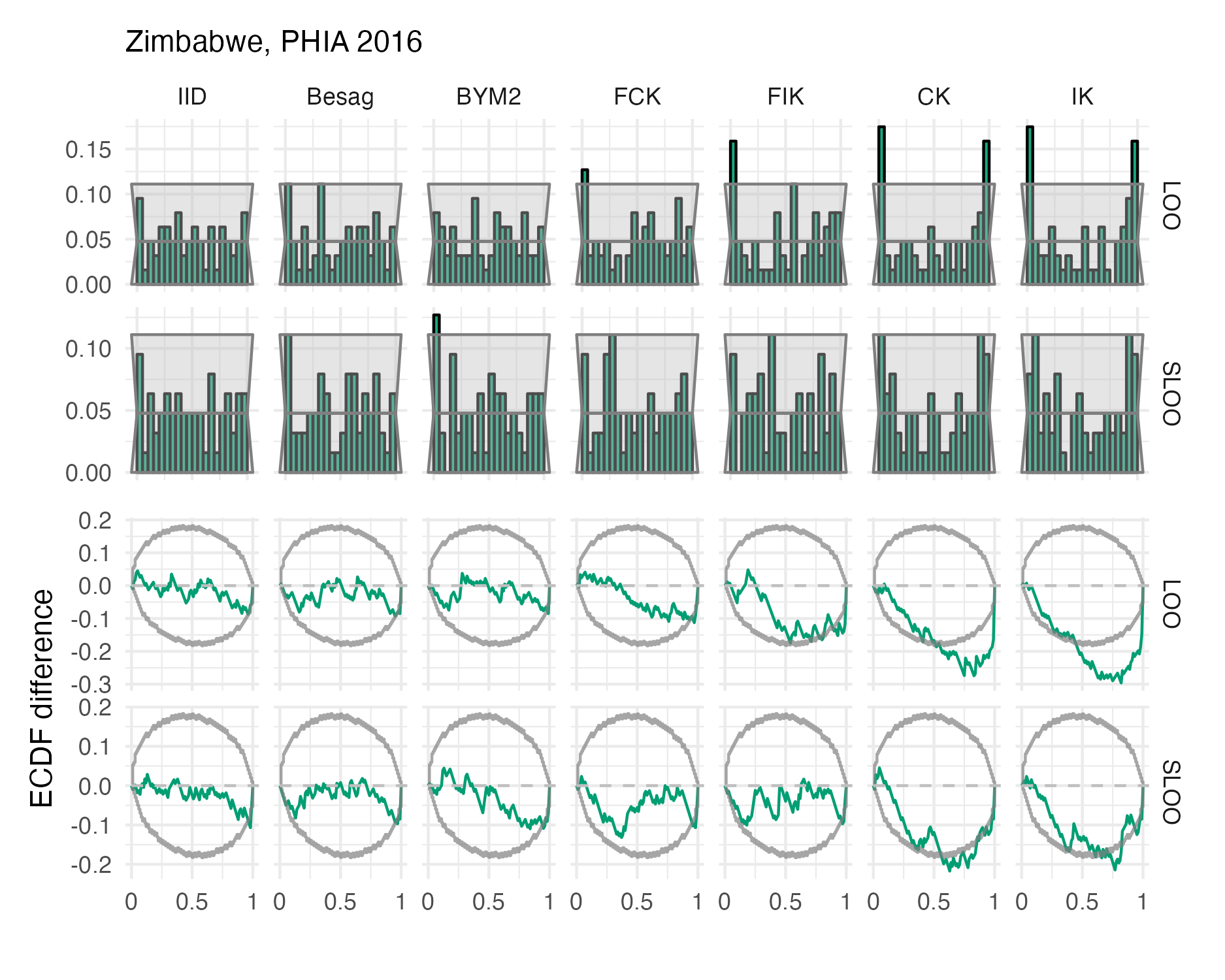
$Probability integral transform histograms and empirical cumulative distribution function difference plots in estimating $\rho$ for the Zimbabwe 2016 PHIA survey (Panel 4.10D).$

Figure A.48: Probability integral transform histograms and empirical cumulative distribution function difference plots in estimating $\rho$ for the Zimbabwe 2016 PHIA survey (Panel 4.10D).

References

Best, N, N Arnold, A Thomas, L Waller, and E Conlon. 1999. “Bayesian models for spatially correlated disease and exposure data.” In Bayesian Statistics 6: Proceedings of the Sixth Valencia International Meeting, 6:131. Oxford University Press.

Betancourt, Michael. 2017. “Robust Gaussian processes in Stan.” https://betanalpha.github.io/assets/case\%5Fstudies/gp\%5Fpart3/part3.html.

Description	Prior	Additional details
Gamma	\(l \sim \text{Gamma}(1, 1)\)	\(-\)
Geometry-informed inverse-gamma	\(l \sim \text{IG}(a, b)\)	The parameters \(a\) and \(b\) chosen such that 5% of the prior mass was below and above the 5% and 95% quantile for distance between points (Betancourt 2017)
Geometry-informed normal	\(l \sim \mathcal{N}^{+}(0, \sigma)\)	The parameter \(\sigma\) set as one third the difference between the minimum and maximum distance between points (Betancourt 2017)
Log-normal	\(l \sim \text{Log-normal}(0, 1)\)	\(-\)
Non-informative	\(p(l) = 1\)	This is an improper prior in that it does not integrate to one
Oracle normal	\(l \sim \mathcal{N}^{+}(2.5, 1)\)	The mean of this prior was set to the true value of the lengthscale