C Fast approximate Bayesian inference

C.1 Epilepsy example

C.1.1 TMB C++ template

// epil.cpp

#include <TMB.hpp>

template <class Type>
Type objective_function<Type>::operator()()
{
  DATA_INTEGER(N);
  DATA_INTEGER(J);
  DATA_INTEGER(K);
  DATA_MATRIX(X);
  DATA_VECTOR(y);
  DATA_MATRIX(E); // Epsilon matrix
  
  PARAMETER_VECTOR(beta);
  PARAMETER_VECTOR(epsilon);
  PARAMETER_VECTOR(nu);
  PARAMETER(l_tau_epsilon);
  PARAMETER(l_tau_nu);
  
  Type tau_epsilon = exp(l_tau_epsilon);
  Type tau_nu = exp(l_tau_nu);
  Type sigma_epsilon = sqrt(1 / tau_epsilon);
  Type sigma_nu = sqrt(1 / tau_nu);
  vector<Type> eta(X * beta + nu + E * epsilon);
  vector<Type> lambda(exp(eta));
  
  Type nll;
  nll = Type(0.0);
  
  // Note: dgamma() is parameterised as (shape, scale)
  // R-INLA is parameterised as (shape, rate)
  nll -= dlgamma(l_tau_epsilon, Type(0.001),
                 Type(1.0 / 0.001), true);
  nll -= dlgamma(l_tau_nu, Type(0.001), Type(1.0 / 0.001), true);
  nll -= dnorm(epsilon, Type(0), sigma_epsilon, true).sum();
  nll -= dnorm(nu, Type(0), sigma_nu, true).sum();
  nll -= dnorm(beta, Type(0), Type(100), true).sum();
  
  nll -= dpois(y, lambda, true).sum();
  
  ADREPORT(tau_epsilon);
  ADREPORT(tau_nu);
  
  return(nll);
}

C.1.2 Modified TMB C++ template

// epil_modified.cpp

#include <TMB.hpp>

template <class Type>
Type objective_function<Type>::operator()()
{
  DATA_INTEGER(N);
  DATA_INTEGER(J);
  DATA_INTEGER(K);
  DATA_MATRIX(X);
  DATA_VECTOR(y);
  DATA_MATRIX(E); // Epsilon matrix
  
  DATA_IVECTOR(x_starts);  // Start index of each subvector of x
  DATA_IVECTOR(x_lengths); // Length of each subvector of x
  DATA_INTEGER(i);         // Index i
  
  PARAMETER(x_i);
  PARAMETER_VECTOR(x_minus_i);
  
  vector<Type> x(301);
  int k = 0;
  for (int j = 0; j < 301; j++) {
    if (j + 1 == i) { // +1 because C++ does zero-indexing
      x(j) = x_i;
    } else {
      x(j) = x_minus_i(k);
      k++;
    }
  }
  
  vector<Type> beta = x.segment(x_starts(0), x_lengths(0));
  vector<Type> epsilon = x.segment(x_starts(1), x_lengths(1));
  vector<Type> nu = x.segment(x_starts(2), x_lengths(2));

  PARAMETER(l_tau_epsilon);
  PARAMETER(l_tau_nu);
  
  Type tau_epsilon = exp(l_tau_epsilon);
  Type tau_nu = exp(l_tau_nu);
  Type sigma_epsilon = sqrt(1 / tau_epsilon);
  Type sigma_nu = sqrt(1 / tau_nu);
  vector<Type> eta(X * beta + nu + E * epsilon);
  vector<Type> lambda(exp(eta));
  
  Type nll;
  nll = Type(0.0);
  
  // Note: dgamma() is parameterised as (shape, scale)
  // R-INLA is parameterised as (shape, rate)
  nll -= dlgamma(l_tau_epsilon, Type(0.001),
                 Type(1.0 / 0.001), true);
  nll -= dlgamma(l_tau_nu, Type(0.001), Type(1.0 / 0.001), true);
  nll -= dnorm(epsilon, Type(0), sigma_epsilon, true).sum();
  nll -= dnorm(nu, Type(0), sigma_nu, true).sum();
  nll -= dnorm(beta, Type(0), Type(100), true).sum();
  
  nll -= dpois(y, lambda, true).sum();
  
  ADREPORT(tau_epsilon);
  ADREPORT(tau_nu);
  
  return(nll);
}

C.1.3 Stan C++ template

// epil.stan

data {
  int<lower=0> N;        // Number of patients
  int<lower=0> J;        // Number of clinic visits
  int<lower=0> K;        // Number of predictors (inc. intercept)
  matrix[N * J, K] X;    // Design matrix
  int<lower=0> y[N * J]; // Outcome variable
  matrix[N * J, N] E;    // Epsilon matrix
}

parameters {
  vector[K] beta;            // Vector of coefficients
  vector[N] epsilon;         // Patient specific errors
  vector[N * J] nu;          // Patient-visit errors
  real<lower=0> tau_epsilon; // Precision of epsilon
  real<lower=0> tau_nu;      // Precision of nu
}

transformed parameters {
  vector[N * J] eta = X * beta + nu + E * epsilon;
}

model {
  beta ~ normal(0, 100);
  tau_epsilon ~ gamma(0.001, 0.001);
  tau_nu ~ gamma(0.001, 0.001);
  epsilon ~ normal(0, sqrt(1 / tau_epsilon));
  nu ~ normal(0, sqrt(1 / tau_nu));
  y ~ poisson_log(eta);
}

C.1.4 NUTS convergence and suitability

C.1.4.1 tmbstan

Traceplots for the tmbstan parameters with the lowest ESS and highest potential scale reduction factor. These were l_tau_nu (an \(\text{ESS}\) of 377) and beta[3] (an \(\hat R\) of 1.006).

Figure C.1: Traceplots for the tmbstan parameters with the lowest ESS and highest potential scale reduction factor. These were l_tau_nu (an \(\text{ESS}\) of 377) and beta[3] (an \(\hat R\) of 1.006).

C.1.4.2 rstan

Traceplots for the rstan parameters with the lowest ESS and highest potential scale reduction factor. These were tau_nu (an \(\text{ESS}\) of 437) and tau_nu (an \(\hat R\) of 1.009). Rather than plotting the traceplot for tau_nu twice, the parameter epsilon[18] is included, which had the second highest \(\hat R\) of 1.008.

Figure C.2: Traceplots for the rstan parameters with the lowest ESS and highest potential scale reduction factor. These were tau_nu (an \(\text{ESS}\) of 437) and tau_nu (an \(\hat R\) of 1.009). Rather than plotting the traceplot for tau_nu twice, the parameter epsilon[18] is included, which had the second highest \(\hat R\) of 1.008.

C.2 Loa loa example

C.2.1 NUTS convergence and suitability

Traceplots for the parameters with the lowest ESS and highest potential scale reduction factor for the Loa loa ELGM example.

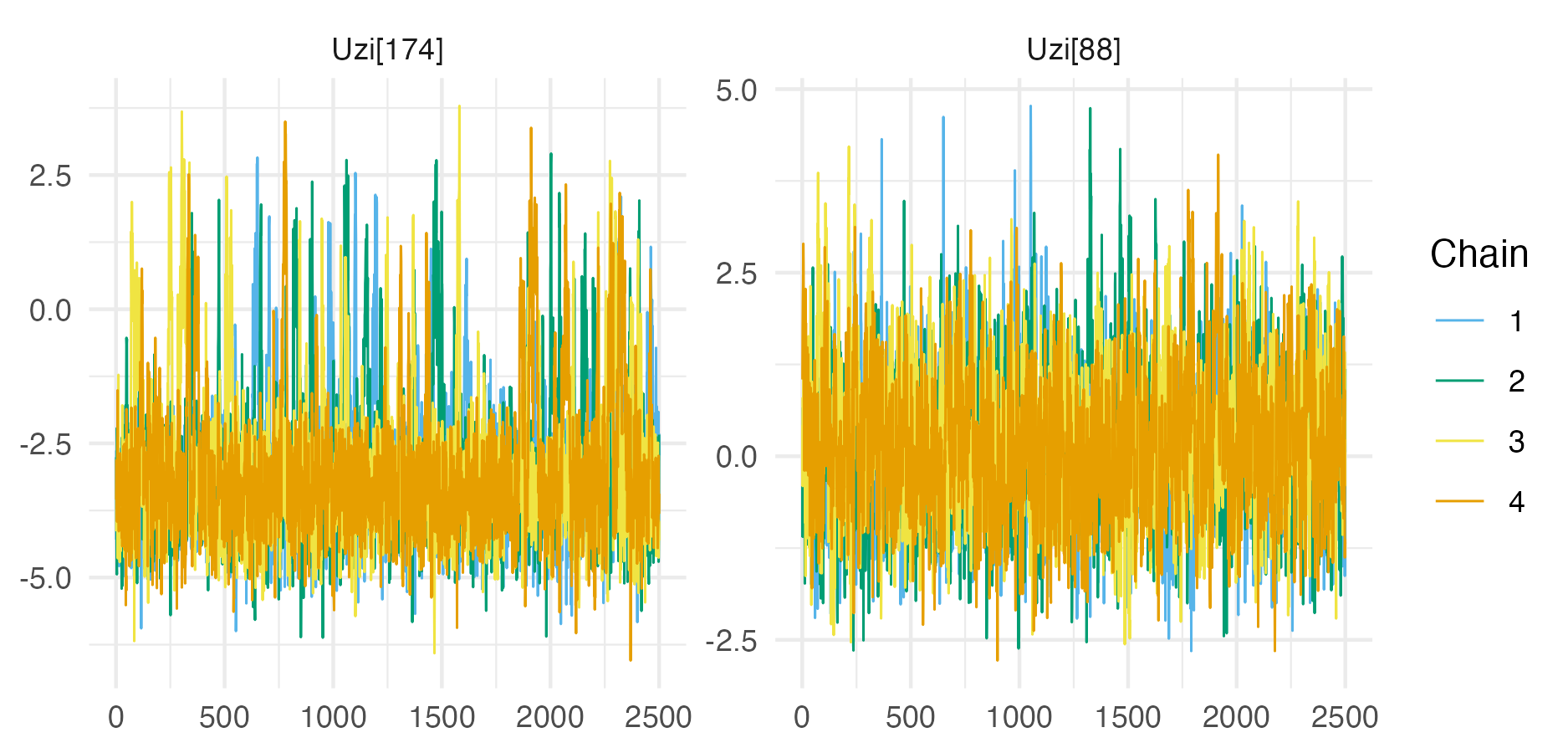
Figure C.3: Traceplots for the parameters with the lowest ESS and highest potential scale reduction factor for the Loa loa ELGM example.

C.2.2 Inference comparison

Relative difference between the Gaussian and Laplace marginal posterior means and standard deviations to NUTS results at each \(u(s_i), v(s_i): i \in [190]\). Absolute differences are in Figure 6.14.

Figure C.4: Relative difference between the Gaussian and Laplace marginal posterior means and standard deviations to NUTS results at each \(u(s_i), v(s_i): i \in [190]\). Absolute differences are in Figure 6.14.

C.3 AGHQ with Laplace marginals algorithm

This section provides the INLA-like algorithm for AGHQ with Laplace marginals used in this thesis. The algorithm for AGHQ with Gaussian marginals used in this thesis is as given in Stringer, Brown, and Stafford (2022), and implemented in the aghq package.

  1. Calculate the mode, Hessian at the mode, lower Cholesky, and Laplace approximation \[\begin{align} \hat{\boldsymbol{\mathbf{\theta}}} &= \arg \max_{\boldsymbol{\mathbf{\theta}}} {\tilde p_\texttt{LA}(\boldsymbol{\mathbf{\theta}}, \mathbf{y})}, \\ \hat{\mathbf{H}} &= - \frac{\partial^2}{\partial \boldsymbol{\mathbf{\theta}} \partial \boldsymbol{\mathbf{\theta}}^\top} \log \tilde p_\texttt{LA}(\boldsymbol{\mathbf{\theta}}, \mathbf{y}) \rvert_{\boldsymbol{\mathbf{\theta}} = \hat{\boldsymbol{\mathbf{\theta}}}}, \\ \hat{\mathbf{H}}^{-1} &= \hat{\mathbf{L}} \hat{\mathbf{L}}^\top, \\ \tilde p_\texttt{LA}(\boldsymbol{\mathbf{\theta}}, \mathbf{y}) &= \frac{p(\mathbf{y}, \mathbf{x}, \boldsymbol{\mathbf{\theta}})}{\tilde p_\texttt{G}(\mathbf{x} \, | \, \boldsymbol{\mathbf{\theta}}, \mathbf{y})} \Big\rvert_{\mathbf{x} = \hat{\mathbf{x}}(\boldsymbol{\mathbf{\theta}})}, \end{align}\] where \(\tilde p_\texttt{G}(\mathbf{x} \, | \, \boldsymbol{\mathbf{\theta}}, \mathbf{y}) = \mathcal{N}(\mathbf{x} \, | \, \hat{\mathbf{x}}(\boldsymbol{\mathbf{\theta}}), \hat{\mathbf{H}}(\boldsymbol{\mathbf{\theta}})^{-1})\) is a Gaussian approximation to \(p(\mathbf{x} \, | \, \boldsymbol{\mathbf{\theta}}, \mathbf{y})\) with mode and precision matrix given by \[\begin{align} \hat{\mathbf{x}}(\boldsymbol{\mathbf{\theta}}) &= \arg \max_\mathbf{x} \log p(\mathbf{y}, \mathbf{x}, \boldsymbol{\mathbf{\theta}}), \\ \hat{\mathbf{H}}(\boldsymbol{\mathbf{\theta}}) &= - \frac{\partial^2}{\partial \mathbf{x} \partial \mathbf{x}^\top} \log p(\mathbf{y}, \mathbf{x}, \boldsymbol{\mathbf{\theta}}) \rvert_{\mathbf{x} = \hat{\mathbf{x}}(\boldsymbol{\mathbf{\theta}})}. \end{align}\]

  2. Generate a set of nodes \(\mathbf{u} \in \mathcal{Q}(m, k)\) and weights \(\omega: \mathbf{u} \to \mathbb{R}\) from a Gauss-Hermite quadrature rule with \(k\) nodes per dimension. Adapt these nodes based on the mode and lower Choleksy via \(\boldsymbol{\mathbf{\theta}}(\mathbf{u}) = \hat{\boldsymbol{\mathbf{\theta}}} + \mathbf{L} \mathbf{u}\). Use this quadrature rule to calculate the normalising constant \(\tilde p_{\texttt{AQ}}(\mathbf{y})\) as follows \[\begin{equation} \tilde p_{\texttt{AQ}}(\mathbf{y}) = \sum_{\mathbf{u} \in \mathcal{Q}(m, k)} \tilde p_\texttt{LA}(\boldsymbol{\mathbf{\theta}}(\mathbf{u}), \mathbf{y}) \omega(\mathbf{u}). \tag{C.1} \end{equation}\]

  3. For \(i \in [N]\) generate \(l\) nodes \(x_i(\mathbf{v})\) via a Gauss-Hermite quadrature rule \(\mathbf{v} \in \mathcal{Q}(1, l)\) adapted based on the mode \(\hat{\mathbf{x}}(\boldsymbol{\mathbf{\theta}})_i\) and standard deviation \(\sqrt{\text{diag}[\hat{\mathbf{H}}(\boldsymbol{\mathbf{\theta}})^{-1}]_i}\) of the Gaussian marginal. A value of \(l \geq 4\) is recommended to enable B-spline interpolation. For \(x_i \in \{ x_i(\mathbf{v}) \}_{\mathbf{v} \in \mathcal{Q}(1, l)}\) and \(\boldsymbol{\mathbf{\theta}} \in \{ \boldsymbol{\mathbf{\theta}}(\mathbf{u}) \}_{\mathbf{u} \in \mathcal{Q}(m, k)}\) calculate the modes and Hessians \[\begin{align} \hat{\mathbf{x}}_{-i}(x_i, \boldsymbol{\mathbf{\theta}}) &= \arg \max_{\mathbf{x}_{-i}} \log p(\mathbf{y}, x_i, \mathbf{x}_{-i}, \boldsymbol{\mathbf{\theta}}), \\ \hat{\mathbf{H}}_{-i, -i}(x_i, \boldsymbol{\mathbf{\theta}}) &= - \frac{\partial^2}{\partial \mathbf{x}_{-i} \partial \mathbf{x}_{-i}^\top} \log p(\mathbf{y}, x_i, \mathbf{x}_{-i}, \boldsymbol{\mathbf{\theta}}) \rvert_{\mathbf{x}_{-i} = \hat{\mathbf{x}}_{-i}(x_i, \boldsymbol{\mathbf{\theta}})}, \end{align}\] where optimisation to obtain \(\hat{\mathbf{x}}_{-i}(x_i, \boldsymbol{\mathbf{\theta}})\) can be initialised at \(\hat{\mathbf{x}}(\boldsymbol{\mathbf{\theta}})_{-i}\).

  4. For \(x_i \in \{ x_i(\mathbf{v}) \}_{\mathbf{v} \in \mathcal{Q}(1, l)}\) calculate \[\begin{equation} p_\texttt{AQ}(x_i \, | \, \mathbf{y}) = \frac{\tilde p_\texttt{LA}(x_i, \mathbf{y})}{\tilde p_{\texttt{AQ}}(\mathbf{y})}, \tag{C.2} \end{equation}\] where \[\begin{equation} \tilde p_\texttt{LA}(x_i, \mathbf{y}) = \sum_{\mathbf{u} \in \mathcal{Q}(m, k)} \tilde p_\texttt{LA}(x_i, \boldsymbol{\mathbf{\theta}}(\mathbf{u}), \mathbf{y}) \omega(\mathbf{u}). \end{equation}\] and \[\begin{equation} \tilde p_\texttt{LA}(x_i, \boldsymbol{\mathbf{\theta}}, \mathbf{y}) = \frac{p(x_i, \mathbf{x}_{-i}, \boldsymbol{\mathbf{\theta}}, \mathbf{y})}{\tilde p_\texttt{G}(\mathbf{x}_{-i} \, | \, x_i, \boldsymbol{\mathbf{\theta}}, \mathbf{y})} \Big\rvert_{\mathbf{x}_{-i} = \hat{\mathbf{x}}_{-i}(x_i, \boldsymbol{\mathbf{\theta}})}. \end{equation}\] Equation (C.2) can be calculated using the estimate of the evidence given in Equation (C.1), but it is more numerically accurate, and requires little extra computation, to use the estimate \[\begin{equation} \tilde p_{\texttt{AQ}}(\mathbf{y}) = \sum_{\mathbf{v} \in \mathcal{Q}(1, l)} \tilde p_\texttt{LA}(x_i(\mathbf{v}), \mathbf{y}) \omega(\mathbf{v}) \end{equation}\]

  5. Given \(\{x_i(\mathbf{v}), \tilde p_\texttt{AQ}(x_i(\mathbf{v}) \, | \, \mathbf{y})\}_{\mathbf{v} \in \mathcal{Q}(1, l)}\) create a spline interpolant to each posterior marginal on the log-scale. Samples, and thereby relevant posterior marginal summaries, may be obtained using inverse transform sampling.

C.4 Simplified Naomi model description

This section describes the simplified version of the Naomi model (Eaton et al. 2021) in more detail. The concise \(i\) indexing used in Section 6.3 is replaced by a more complete \(x, s, a\) indexing. There are four sections:

  1. Section C.4.1 gives the process specifications, giving the terms in each structured additive predictor, along with their distributions.
  2. Section C.4.2 gives additional details about the likelihood terms not provided in Section 6.3.
  3. Section C.4.3 gives identifiability constraints used in circumstances where incomplete data is available for the country.
  4. Section C.4.4 provides details of the TMB implementation.

C.4.1 Process specification

Table C.1: The Naomi model can be conceptualised as having five processes. This table gives the number of latent field parameters and hyperparameters in each process, where \(n\) is the number of districts in the country.
Model component Latent field Hyperparameter
Section C.4.1.1 HIV prevalence \(22 + 5n\) 9
Section C.4.1.2 ART coverage \(25 + 5n\) 9
Section C.4.1.3 HIV incidence rate \(2 + n\) 3
Section C.4.1.4 ANC testing \(2 + 2n\) 2
Section C.4.1.5 ART attendance \(n\) 1
Total \(51 + 14n\) 24

C.4.1.1 HIV prevalence

HIV prevalence \(\rho_{x, s, a} \in [0, 1]\) was modelled on the logit scale using the structured additive predictor \[\begin{equation} \text{logit}(\rho_{x, s, a}) = \beta^\rho_0 + \beta_{S}^{\rho, s = \text{M}} + \mathbf{u}^\rho_a + \mathbf{u}_a^{\rho, s = \text{M}} + \mathbf{u}^\rho_x + \mathbf{u}_x^{\rho, s = \text{M}} + \mathbf{u}_x^{\rho, a < 15} + \boldsymbol{\mathbf{\eta}}^\rho_{R_x, s, a}. \tag{C.3} \end{equation}\] Table C.2 provides a description of the terms included in Equation (C.3). Independent half-normal prior distributions were chosen for the five standard deviation terms \[\begin{equation} \{\sigma_A^\rho, \sigma_{AS}^\rho, \sigma_X^\rho, \sigma_{XS}^\rho, \sigma_{XA}^\rho\} \sim \mathcal{N}^{+}(0, 2.5), \end{equation}\] independent uniform prior distributions for the two AR1 correlation parameters \[\begin{equation} \{\phi_A^\rho, \phi_{AS}^\rho\} \sim \mathcal{U}(-1, 1), \end{equation}\] and independent beta prior distributions for the two BYM2 proportion parameters \[\begin{equation} \{\phi_X^\rho, \phi_{XS}^\rho\} \sim \text{Beta}(0.5, 0.5). \end{equation}\]

Table C.2: Each term in Equation (C.3) together with, where applicable, its prior distribution and a written description of its role.
Term Distribution Description
\(\beta^\rho_0\) \(\mathcal{N}(0, 5)\) Intercept
\(\beta_{s}^{\rho, s = \text{M}}\) \(\mathcal{N}(0, 5)\) The difference in logit prevalence for men compared to women
\(\mathbf{u}^\rho_a\) \(\text{AR}1(\sigma_A^\rho, \phi_A^\rho)\) Age random effects for women
\(\mathbf{u}_a^{\rho, s = \text{M}}\) \(\text{AR}1(\sigma_{AS}^\rho, \phi_{AS}^\rho)\) Age random effects for the difference in logit prevalence for men compared to women age \(a\)
\(\mathbf{u}^\rho_x\) \(\text{BYM}2(\sigma_X^\rho, \phi_X^\rho)\) Spatial random effects for women
\(\mathbf{u}_x^{\rho, s = \text{M}}\) \(\text{BYM}2(\sigma_{XS}^\rho, \phi_{XS}^\rho)\) Spatial random effects for the difference in logit prevalence for men compared to women in district \(x\)
\(\mathbf{u}_x^{\rho, a < 15}\) \(\text{ICAR}(\sigma_{XA}^\rho)\) Spatial random effects for the difference in logit paediatric prevalence to adult women prevalence in district \(x\)
\(\boldsymbol{\mathbf{\eta}}^\rho_{R_x, s, a}\) \(-\) Fixed offsets specifying assumed odds ratios for prevalence outside the age ranges for which data were available. Calculated from Spectrum model (Stover et al. 2019) outputs for region \(R_x\)

C.4.1.2 ART coverage

ART coverage \(\alpha_{x, s, a} \in [0, 1]\) was modelled on the logit scale using the structured additive predictor \[\begin{equation} \text{logit}(\alpha_{x, s, a}) = \beta^\alpha_0 + \beta_{S}^{\alpha, s = \text{M}} + \mathbf{u}^\alpha_a + \mathbf{u}_a^{\alpha, s = \text{M}} + \mathbf{u}^\alpha_x + \mathbf{u}_x^{\alpha, s = \text{M}} + \mathbf{u}_x^{\alpha, a < 15} + \boldsymbol{\mathbf{\eta}}^\alpha_{R_x, s, a} \end{equation}\] with terms and prior distributions analogous to the HIV prevalence process model in Section C.4.1.1 above.

C.4.1.3 HIV incidence rate

HIV incidence rate \(\lambda_{x, s, a} > 0\) was modelled on the log scale using the structured additive predictor \[\begin{equation} \log(\lambda_{x, s, a}) = \beta_0^\lambda + \beta_S^{\lambda, s = \text{M}} + \log(\rho_{x}^{\text{15-49}}) + \log(1 - \omega \cdot \alpha_{x}^{\text{15-49}}) + \mathbf{u}_x^\lambda + \boldsymbol{\mathbf{\eta}}_{R_x, s, a}^\lambda. \tag{C.4} \end{equation}\] Table C.3 provides a description of the terms included in Equation (C.4).

Table C.3: Each term in Equation (C.4) together with, where applicable, its prior distribution and a written description of its role.
Term Distribution Description
\(\beta^\lambda_0\) \(\mathcal{N}(0, 5)\) Intercept term proportional to the average HIV transmission rate for untreated HIV positive adults
\(\beta_S^{\lambda, s = \text{M}}\) \(\mathcal{N}(0, 5)\) The log incidence rate ratio for men compared to women
\(\rho_{x}^{\text{15-49}}\) \(-\) The HIV prevalence among adults 15-49 in district \(x\) calculated by aggregating age-specific HIV prevalences
\(\alpha_{x}^{\text{15-49}}\) \(-\) The ART coverage among adults 15-49 in district \(x\) calculated by aggregating age-specific ART coverages
\(\omega = 0.7\) \(-\) Average reduction in HIV transmission rate per increase in population ART coverage fixed based on inputs to the Estimation and Projection Package (EPP) model
\(\mathbf{u}_x^\lambda\) \(\mathcal{N}(0, \sigma^\lambda)\) IID spatial random effects with \(\sigma^\lambda \sim \mathcal{N}^+(0, 1)\)
\(\boldsymbol{\mathbf{\eta}}^\lambda_{R_x, s, a}\) \(-\) Fixed log incidence rate ratios by sex and age group calculated from Spectrum model outputs for region \(R_x\)

The proportion recently infected among HIV positive persons \(\kappa_{x, s, a} \in [0, 1]\) was modelled as \[\begin{equation} \kappa_{x, s, a} = 1 - \exp \left(- \lambda_{x, s, a} \cdot \frac{1 - \rho_{x, s, a}}{\rho_{x, s, a}} \cdot (\Omega_T - \beta_T ) - \beta_T \right), \end{equation}\] where \(\Omega_T \sim \mathcal{N}(\Omega_{T_0}, \sigma^{\Omega_T})\) is the mean duration of recent infection, and \(\beta_T \sim \mathcal{N}^{+}(\beta_{T_0}, \sigma^{\beta_T})\) is the false recent ratio. The prior distribution for \(\Omega_T\) was informed by the characteristics of the recent infection testing algorithm. For PHIA surveys this was \(\Omega_{T_0} = 130 \text{ days}\) and \(\sigma^{\Omega_T} = 6.12 \text{ days}\). For PHIA surveys there was assumed to be no false recency, such that \(\beta_{T_0} = 0.0\), \(\sigma^{\beta_T} = 0.0\), and \(\beta_T = 0\).

C.4.1.4 ANC testing

HIV prevalence \(\rho_{x, a}^\text{ANC}\) and ART coverage \(\alpha_{x, a}^\text{ANC}\) among pregnant women were modelled as being offset on the logit scale from the corresponding district-age indicators \(\rho_{x, F, a}\) and \(\alpha_{x, F, a}\) according to \[\begin{align} \text{logit}(\rho_{x, a}^{\text{ANC}}) &= \text{logit}(\rho_{x, F, a}) + \beta^{\rho^{\text{ANC}}} + \mathbf{u}_x^{\rho^{\text{ANC}}} + \boldsymbol{\mathbf{\eta}}_{R_x, a}^{\rho^{\text{ANC}}}, \tag{C.5} \\ \text{logit}(\alpha_{x, a}^{\text{ANC}}) &= \text{logit}(\alpha_{x, F, a}) + \beta^{\alpha^{\text{ANC}}} + \mathbf{u}_x^{\alpha^{\text{ANC}}} + \boldsymbol{\mathbf{\eta}}_{R_x, a}^{\alpha^{\text{ANC}}} \tag{C.6}. \end{align}\] Table C.4 provides a description of the terms included in Equation (C.5) and Equation (C.6).

Table C.4: Each term in Equations (C.5) and (C.6) together with (where applicable) its prior distribution and a written description of its role. The notation \(\theta\) is used as stand in for \(\theta \in \{\rho, \alpha\}\).
Term Distribution Description
\(\beta^{\theta^{\text{ANC}}}\) \(\mathcal{N}(0, 5)\) Intercept giving the average difference between population and ANC outcomes
\(\mathbf{u}_x^{\theta^{\text{ANC}}}\) \(\mathcal{N}(0, \sigma_X^{\theta^{\text{ANC}}})\) IID district random effects with \(\sigma_X^{\theta^{\text{ANC}}} \sim \mathcal{N}^+(0, 1)\)
\(\boldsymbol{\mathbf{\eta}}_{R_x, a}^{\theta^{\text{ANC}}}\) \(-\) Offsets for the log fertility rate ratios for HIV positive women compared to HIV negative women and for women on ART to HIV positive women not on ART, calculated from Spectrum model outputs for region \(R_x\)

In the full Naomi model, for adult women 15-49 the number of ANC clients \(\Psi_{x, a} > 0\) were modelled as \[\begin{equation} \log (\Psi_{x, a}) = \log (N_{x, \text{F}, a}) + \psi_{R_x, a} + \beta^\psi + \mathbf{u}_x^\psi, \end{equation}\] where \(N_{x, \text{F}, a}\) are the female population sizes, \(\psi_{R_x, a}\) are fixed age-sex fertility ratios in Spectrum region \(R_x\), \(\beta^\psi\) are log rate ratios for the number of ANC clients relative to the predicted fertility, and \(\mathbf{u}_x^\psi \sim \mathcal{N}(0, \sigma^\psi)\) are district random effects. Here these terms are fixed to \(\beta^\psi = 0\) and \(\mathbf{u}_x^\psi = \mathbf{0}\) such that \(\Psi_{x, a}\) are simply constants.

C.4.1.5 ART attendance

Let \(\gamma_{x, x'} \in [0, 1]\) be the probability that a person on ART residing in district \(x\) receives ART in district \(x'\). Assume that \(\gamma_{x, x'} = 0\) for \(x \notin \{x, \text{ne}(x)\}\) such that individuals seek treatment only in their residing district or its neighbours \(\text{ne}(x) = \{x': x' \sim x\}\), where \(\sim\) is an adjacency relation, and \(\sum_{x' \in \{x, \text{ne}(x)\}} \gamma_{x, x'} = 1\).

The probabilities \(\gamma_{x, x'}\) for \(x \sim x'\) were modelled using multinomial logistic regression model, based on the log-odds ratios \[\begin{equation} \tilde \gamma_{x, x'} = \log \left( \frac{\gamma_{x, x'}}{1 - \gamma_{x, x'}} \right) = \tilde \gamma_0 + \mathbf{u}_x^{\tilde \gamma}. \tag{C.7} \end{equation}\] Table C.5 provides a description of the terms included in Equation (C.7). Fixing \(\tilde \gamma_{x, x} = 0\) then the multinomial probabilities may be recovered using the softmax \[\begin{equation} \gamma_{x, x'} = \frac{\exp(\tilde \gamma_{x, x'})}{\sum_{x^\star \in \{x, \text{ne}(x)\}} \exp(\tilde \gamma_{x, x^\star})}. \end{equation}\]

Table C.5: Each term in Equation (C.7) together with, where applicable, its prior distribution and a written description of its role. As no terms include \(x'\), \(\gamma_{x, x'}\) is only a function of \(x\).
Term Distribution Description
\(\tilde \gamma_0\) \(-\) Fixed intercept \(\tilde \gamma_0 = -4\). Implies a prior mean on \(\gamma_{x, x'}\) of 1.8%, such that a-priori \((100 - 1.8 \times \text{ne}(x))\%\) of ART clients in district \(x\) obtain treatment in their home district
\(\mathbf{u}_x^{\tilde \gamma}\) \(\mathcal{N}(0, \sigma_X^{\tilde \gamma})\) District random effects, with \(\sigma_X^{\tilde \gamma} \sim \mathcal{N}^+(0, 2.5)\)

C.4.2 Additional likelihood specification

Though Section 6.3 provides a complete description of Naomi’s likelihood specification, any additional useful details are provided here.

C.4.2.1 Household survey data

The generalised binomial \(y \sim \text{xBin}(m, p)\) is defined for \(y, m \in \mathbb{R}^+\) with \(y \leq m\) such that \[\begin{align} \log p(y) = &\log \Gamma(m + 1) - \log \Gamma(y + 1) \\ &- \log \Gamma(m - y + 1) + y \log p + (m - y) \log(1 - p), \end{align}\] where the gamma function \(\Gamma\) is such that \(\forall n \in \mathbb{N}\), \(\Gamma(n) = (n - 1)!\).

C.4.3 Identifiability constraints

If data are missing, some parameters are fixed to default values to help with identifiability. In particular:

  1. If survey data on HIV prevalence or ART coverage by age and sex are not available then \(\mathbf{u}_a^\theta = 0\) and \(\mathbf{u}_{a, s = \text{M}}^\theta = 0\). In this case, the average age-sex pattern from the Spectrum is used. For the Malawi case-study (Section 6.5), HIV prevalence and ART coverage data are not available for those aged 65+. As a result, there are \(|\{\text{0-4}, \ldots, \text{50-54}\}| = 13\) age groups included for the age random effects.
  2. If no ART data, either survey or ART programme, are available but data on ART coverage among ANC clients are available, the level of ART coverage is not identifiable, but spatial variation is identifiable. In this instance, overall ART coverage is determined by the Spectrum offset, and only area random effects are estimated such that \[\begin{equation} \text{logit} \left(\alpha_{x, s, a} \right) = \mathbf{u}_x^\alpha + \boldsymbol{\mathbf{\eta}}_{R_x, s, a}^\alpha. \end{equation}\]
  3. If survey data on recent HIV infection are not included in the model, then \(\beta_0^\lambda = \beta_S^{\lambda, s = \text{M}} = 0\) and \(\mathbf{u}_x^\lambda = \mathbf{0}\). The sex ratio for HIV incidence is determined by the sex incidence rate ratio from Spectrum, and the incidence rate in all districts is modelled assuming the same average HIV transmission rate for untreated adults, but varies according to district-level estimates of HIV prevalence and ART coverage.

C.4.4 Implementation

The TMB C++ code for the negative log-posterior of the simplified Naomi model is available from https://github.com/athowes/naomi-aghq. For ease of understanding, Table C.6 provides correspondence between the mathematical notation used in Section C.4 and the variable names used in the TMB code, for all hyperparameters and latent field parameters. For further reference on the TMB software see Kristensen (2021).

Table C.6: Correspondence between the variable name used in the Naomi TMB template and the mathematical notation used in Appendix C.4. The parameter type, either a hyperparameter or element of the latent field, is also given. All of the parameters are defined on the real-scale in some dimension. In the final three columns (\(\rho\), \(\alpha\), and \(\lambda\)) indication is given as to which component of the model the parameter is primarily used in.
Variable name Notation Type Domain \(\rho\) \(\alpha\) \(\lambda\)
logit_phi_rho_x \(\text{logit}(\phi_X^\rho)\) Hyper \(\mathbb{R}\) Yes
log_sigma_rho_x \(\log(\sigma_X^\rho)\) Hyper \(\mathbb{R}\) Yes
logit_phi_rho_xs \(\text{logit}(\phi_{XS}^\rho)\) Hyper \(\mathbb{R}\) Yes
log_sigma_rho_xs \(\log(\sigma_{XS}^\rho)\) Hyper \(\mathbb{R}\) Yes
logit_phi_rho_a \(\text{logit}(\phi_A^\rho)\) Hyper \(\mathbb{R}\) Yes
log_sigma_rho_a \(\log(\sigma_A^\rho)\) Hyper \(\mathbb{R}\) Yes
logit_phi_rho_as \(\text{logit}(\phi_{AS}^\rho)\) Hyper \(\mathbb{R}\) Yes
log_sigma_rho_as \(\log(\sigma_{AS}^\rho)\) Hyper \(\mathbb{R}\) Yes
log_sigma_rho_xa \(\log(\sigma_{XA}^\rho)\) Hyper \(\mathbb{R}\) Yes
logit_phi_alpha_x \(\text{logit}(\phi_X^\alpha)\) Hyper \(\mathbb{R}\) Yes
log_sigma_alpha_x \(\log(\sigma_X^\alpha)\) Hyper \(\mathbb{R}\) Yes
logit_phi_alpha_xs \(\text{logit}(\phi_{XS}^\alpha)\) Hyper \(\mathbb{R}\) Yes
log_sigma_alpha_xs \(\log(\sigma_{XS}^\alpha)\) Hyper \(\mathbb{R}\) Yes
logit_phi_alpha_a \(\text{logit}(\phi_A^\alpha)\) Hyper \(\mathbb{R}\) Yes
log_sigma_alpha_a \(\log(\sigma_A^\alpha)\) Hyper \(\mathbb{R}\) Yes
logit_phi_alpha_as \(\text{logit}(\phi_{AS}^\alpha)\) Hyper \(\mathbb{R}\) Yes
log_sigma_alpha_as \(\log(\sigma_{AS}^\alpha)\) Hyper \(\mathbb{R}\) Yes
log_sigma_alpha_xa \(\log(\sigma_{XA}^\alpha)\) Hyper \(\mathbb{R}\) Yes
OmegaT_raw \(\Omega_T\) Hyper \(\mathbb{R}\) Yes
log_betaT \(\log(\beta_T)\) Hyper \(\mathbb{R}\) Yes
log_sigma_lambda_x \(\log(\sigma^\lambda)\) Hyper \(\mathbb{R}\) Yes
log_sigma_ancrho_x \(\log(\sigma_X^{\rho^{\text{ANC}}})\) Hyper \(\mathbb{R}\) Yes
log_sigma_ancalpha_x \(\log(\sigma_X^{\alpha^{\text{ANC}}})\) Hyper \(\mathbb{R}\) Yes
log_sigma_or_gamma \(\log(\sigma_X^{\tilde \gamma})\) Hyper \(\mathbb{R}\)
beta_rho \((\beta^\rho_0, \beta_{s}^{\rho, s = \text{M}})\) Latent \(\mathbb{R}^2\) Yes
beta_alpha \((\beta^\alpha_0, \beta_{S}^{\alpha, s = \text{M}})\) Latent \(\mathbb{R}^2\) Yes
beta_lambda \((\beta_0^\lambda, \beta_S^{\lambda, s = \text{M}})\) Latent \(\mathbb{R}^2\) Yes
beta_anc_rho \(\beta^{\rho^{\text{ANC}}}\) Latent \(\mathbb{R}\) Yes
beta_anc_alpha \(\beta^{\alpha^{\text{ANC}}}\) Latent \(\mathbb{R}\) Yes
u_rho_x \(\mathbf{w}^\rho_x\) Latent \(\mathbb{R}^{n}\) Yes
us_rho_x \(\mathbf{v}^\rho_x\) Latent \(\mathbb{R}^{n}\) Yes
u_rho_xs \(\mathbf{w}_x^{\rho, s = \text{M}}\) Latent \(\mathbb{R}^{n}\) Yes
us_rho_xs \(\mathbf{v}_x^{\rho, s = \text{M}}\) Latent \(\mathbb{R}^{n}\) Yes
u_rho_a \(\mathbf{u}^\rho_a\) Latent \(\mathbb{R}^{10}\) Yes
u_rho_as \(\mathbf{u}_a^{\rho, s = \text{M}}\) Latent \(\mathbb{R}^{10}\) Yes
u_rho_xa \(\mathbf{u}_x^{\rho, a < 15}\) Latent \(\mathbb{R}^{n}\) Yes
u_alpha_x \(\mathbf{w}^\alpha_x\) Latent \(\mathbb{R}^{n}\) Yes
us_alpha_x \(\mathbf{v}^\alpha_x\) Latent \(\mathbb{R}^{n}\) Yes
u_alpha_xs \(\mathbf{w}_x^{\alpha, s = \text{M}}\) Latent \(\mathbb{R}^{n}\) Yes
us_alpha_xs \(\mathbf{v}_x^{\alpha, s = \text{M}}\) Latent \(\mathbb{R}^{n}\) Yes
u_alpha_a \(\mathbf{u}^\alpha_a\) Latent \(\mathbb{R}^{13}\) Yes
u_alpha_as \(\mathbf{u}_a^{\alpha, s = \text{M}}\) Latent \(\mathbb{R}^{10}\) Yes
u_alpha_xa \(\mathbf{u}_x^{\alpha, a < 15}\) Latent \(\mathbb{R}^{n}\) Yes
ui_lambda_x \(\mathbf{u}_x^\lambda\) Latent \(\mathbb{R}^{n}\) Yes
ui_anc_rho_x \(\mathbf{u}_x^{\rho^{\text{ANC}}}\) Latent \(\mathbb{R}^{n}\) Yes
ui_anc_alpha_x \(\mathbf{u}_x^{\alpha^{\text{ANC}}}\) Latent \(\mathbb{R}^{n}\) Yes
log_or_gamma \(\mathbf{u}_x^{\tilde \gamma}\) Latent \(\mathbb{R}^{n}\)

C.5 NUTS convergence and suitability

For NUTS run on the Naomi ELGM, the maximum potential scale reduction factor was 1.021, below the value of 1.05 typically used as a cutoff for acceptable chain mixing, indicating that the results are acceptable to use. Additionally, the vast majority (93.7%) of \(\hat R\) values were less than 1.1.

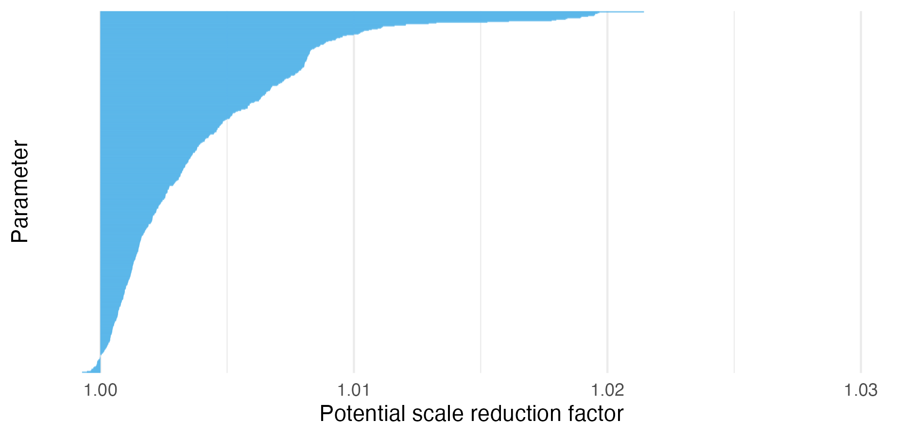
Figure C.5: For NUTS run on the Naomi ELGM, the maximum potential scale reduction factor was 1.021, below the value of 1.05 typically used as a cutoff for acceptable chain mixing, indicating that the results are acceptable to use. Additionally, the vast majority (93.7%) of \(\hat R\) values were less than 1.1.

The efficiency of the NUTS, as measured by the ratio of effective sample size to total number of iterations run, was low for most parameters (Panel A). As a result, the number of iterations required for the the effective number of samples (mean 1265) to be satisfactory was high (Panel B).

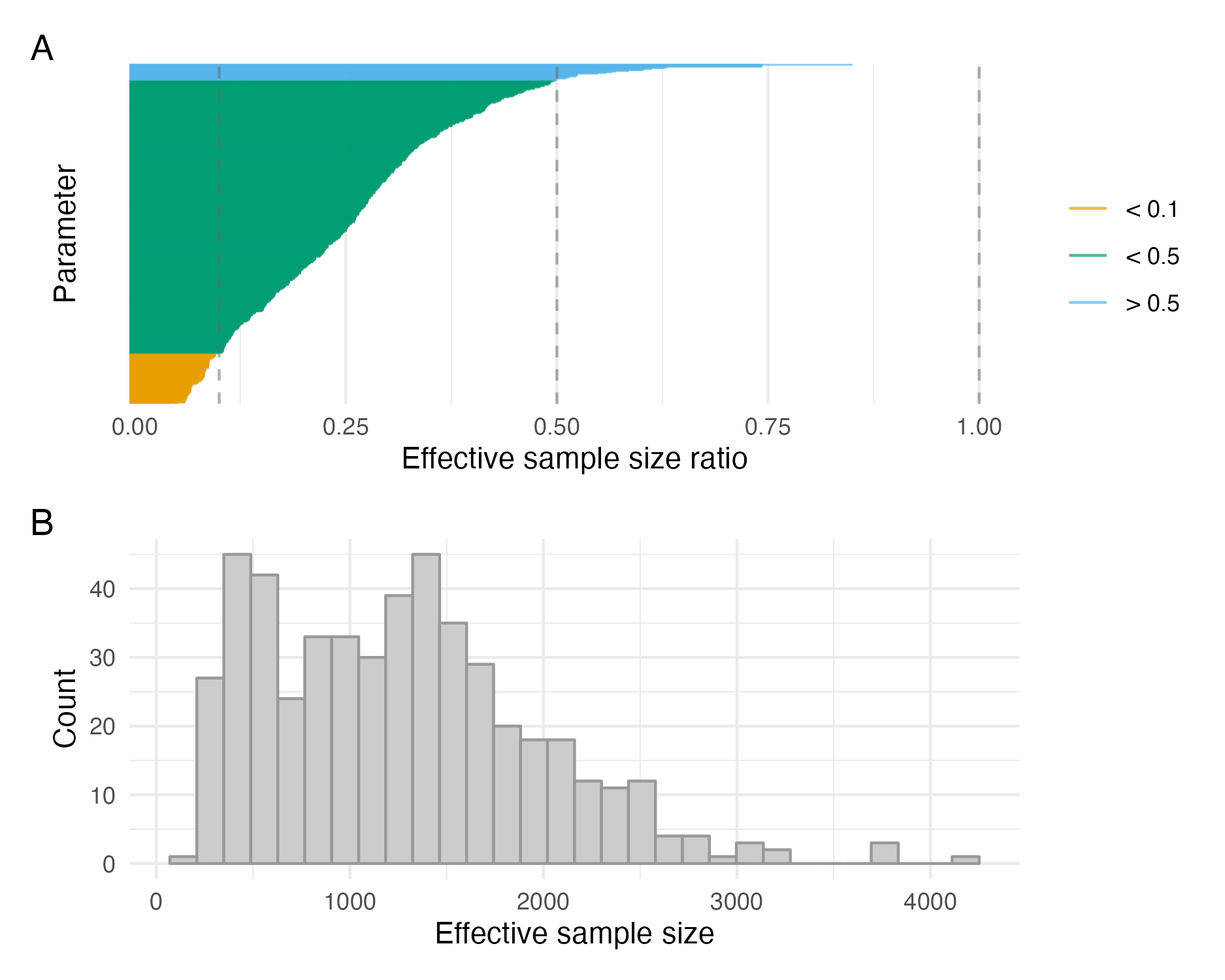
Figure C.6: The efficiency of the NUTS, as measured by the ratio of effective sample size to total number of iterations run, was low for most parameters (Panel A). As a result, the number of iterations required for the the effective number of samples (mean 1265) to be satisfactory was high (Panel B).

Traceplots for the parameter with the lowest ESS which was log_sigma_alpha_xs (an \(\text{ESS}\) of 208, Panel A) and highest potential scale reduction factor which was ui_lambda_x[10] (an \(\hat R\) of 1.021, Panel B).

Figure C.7: Traceplots for the parameter with the lowest ESS which was log_sigma_alpha_xs (an \(\text{ESS}\) of 208, Panel A) and highest potential scale reduction factor which was ui_lambda_x[10] (an \(\hat R\) of 1.021, Panel B).

Pairs plots for the parameters \(\log(\sigma_{A}^\rho)\) and \(\text{logit}(\phi_{A}^\rho)\), or log_sigma_rho_a and logit_phi_rho_a as implemented in code. These parameters are the log standard deviation and logit lag-one correlation parameter of an AR1 process. In the posterior distribution obtained with NUTS, they have a high degree of correlation.

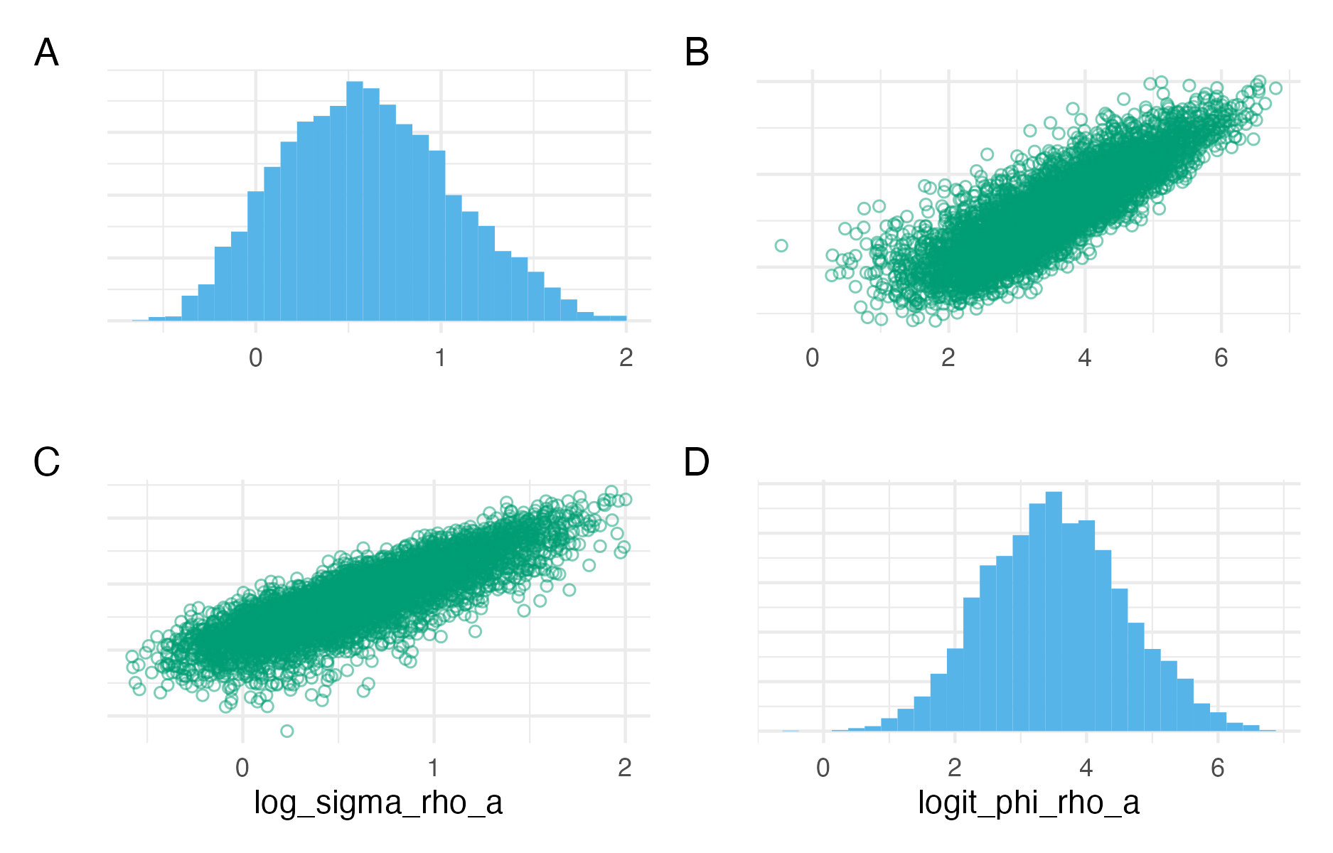
Figure C.8: Pairs plots for the parameters \(\log(\sigma_{A}^\rho)\) and \(\text{logit}(\phi_{A}^\rho)\), or log_sigma_rho_a and logit_phi_rho_a as implemented in code. These parameters are the log standard deviation and logit lag-one correlation parameter of an AR1 process. In the posterior distribution obtained with NUTS, they have a high degree of correlation.

Pairs plots for the parameters \(\log(\sigma_X^\alpha)\) and \(\text{logit}(\phi_X^\alpha)\), or log_sigma_alpha_x and logit_phi_alpha_x as implemented in code. These parameters are the log standard deviation and logit BYM2 proportion parameter of a BYM2 process. In the posterior distribution obtained with NUTS, they are close to uncorrelated.

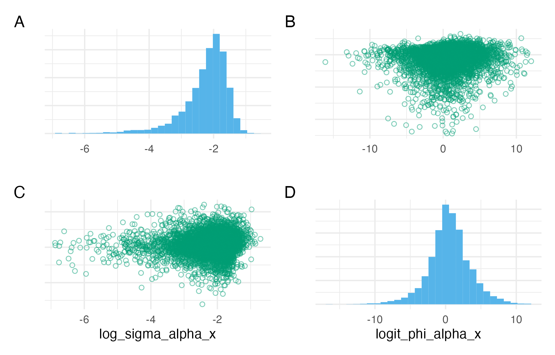
Figure C.9: Pairs plots for the parameters \(\log(\sigma_X^\alpha)\) and \(\text{logit}(\phi_X^\alpha)\), or log_sigma_alpha_x and logit_phi_alpha_x as implemented in code. These parameters are the log standard deviation and logit BYM2 proportion parameter of a BYM2 process. In the posterior distribution obtained with NUTS, they are close to uncorrelated.

Prior standard deviations were calculated by using NUTS to simulate from the prior distribution. This approach is more convenient than simulating directly from the model, but can lead to inaccuracies.

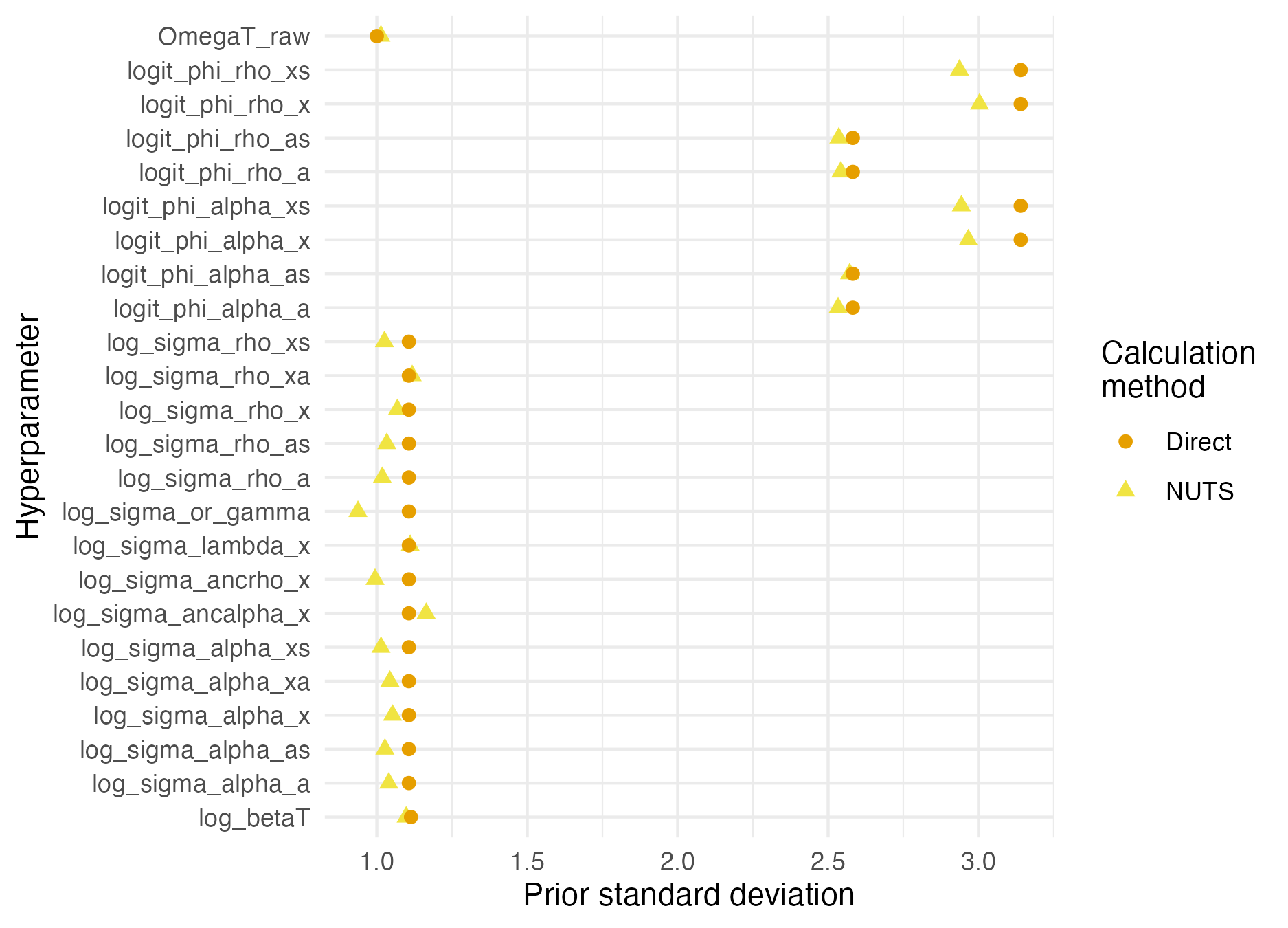
Figure C.10: Prior standard deviations were calculated by using NUTS to simulate from the prior distribution. This approach is more convenient than simulating directly from the model, but can lead to inaccuracies.

The posterior contraction for each parameter in the model. Values are averaged for parameters of length greater than one. The posterior contraction is zero when the prior distribution and posterior distribution have the same standard deviation. This could indicate that the data is not informative about the parameter. The closer the posterior contraction is to one, the more than the marginal posterior distribution has concentrated about a single point.

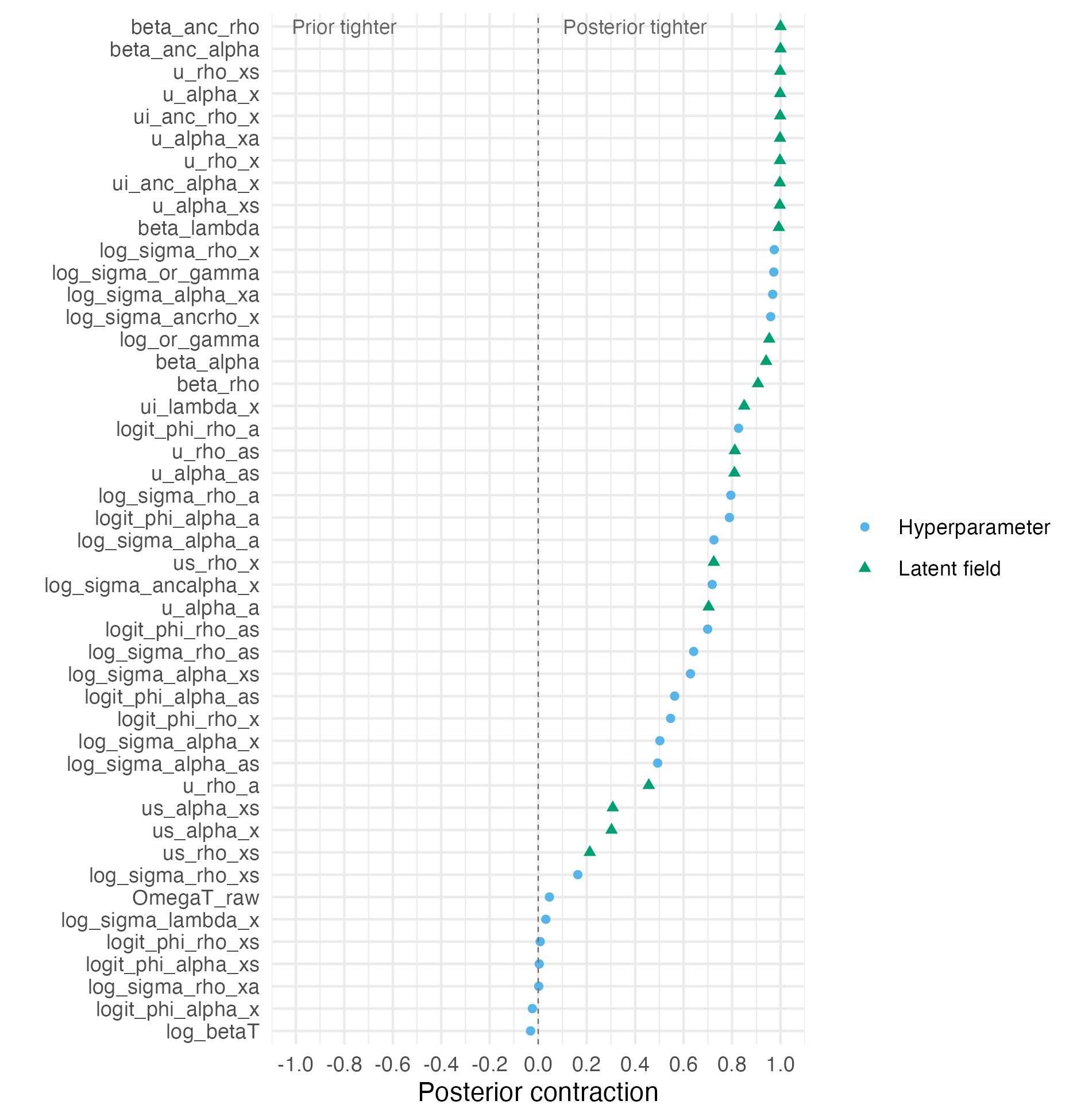
Figure C.11: The posterior contraction for each parameter in the model. Values are averaged for parameters of length greater than one. The posterior contraction is zero when the prior distribution and posterior distribution have the same standard deviation. This could indicate that the data is not informative about the parameter. The closer the posterior contraction is to one, the more than the marginal posterior distribution has concentrated about a single point.

C.6 Use of PCA-AGHQ

The standard deviation of the quadrature nodes can be used as a measure of coverage of the posterior marginal distribution. Nodes spaced evenly within the marginal distribution would be expected to uniformly distributed quantile, corresponding to a standard deviation of 0.2861, shown as a dashed line.

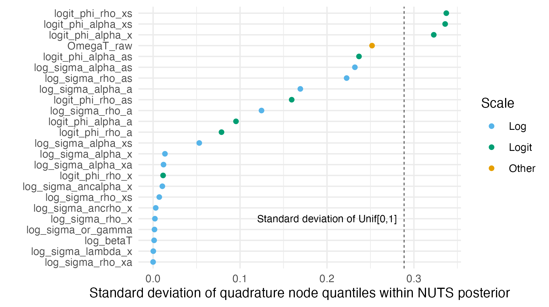
Figure C.12: The standard deviation of the quadrature nodes can be used as a measure of coverage of the posterior marginal distribution. Nodes spaced evenly within the marginal distribution would be expected to uniformly distributed quantile, corresponding to a standard deviation of 0.2861, shown as a dashed line.

The estimated posterior marginal standard deviation of each hyperparameter varied substantially based on its scale, either logarithmic or logistic.

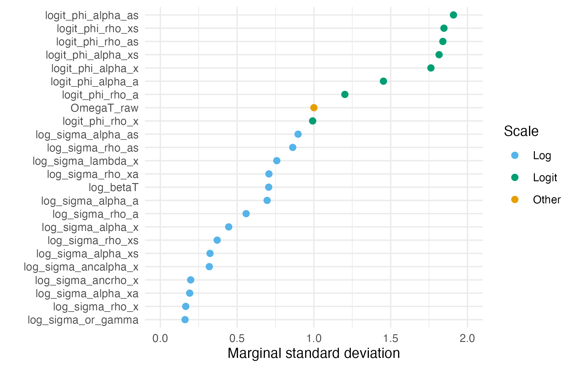
Figure C.13: The estimated posterior marginal standard deviation of each hyperparameter varied substantially based on its scale, either logarithmic or logistic.

The logarithm of the normalising constant estimated using PCA-AGHQ and a range of possible values of \(k = 2, 3, 5\) and \(s \leq 8\). Using this range of settings, there was not convergence of the logarithm of the normalsing constant estimate. The time taken by GPCA-AGHQ increases exponentially with number of PCA-AGHQ dimensions kept.

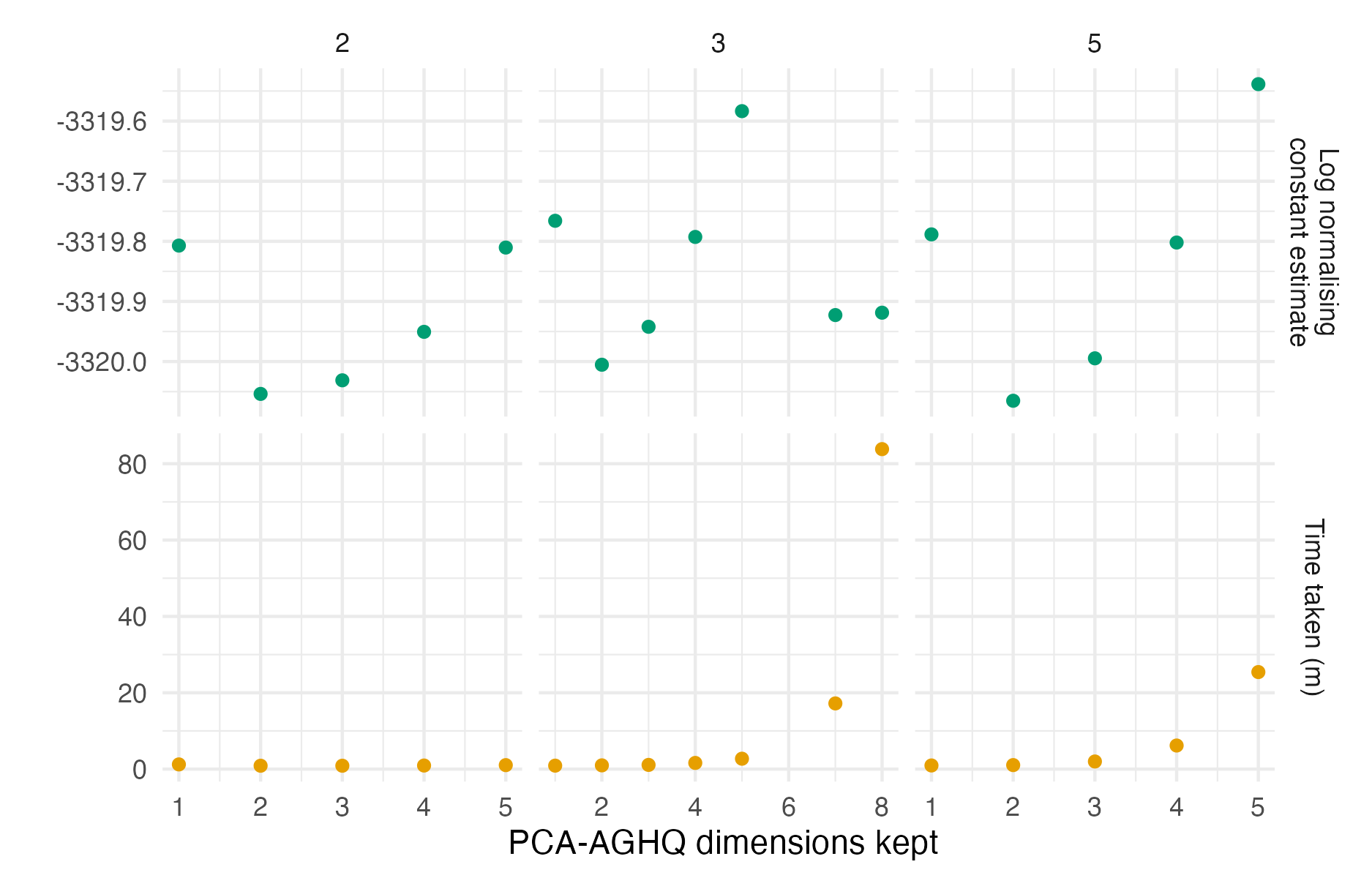
Figure C.14: The logarithm of the normalising constant estimated using PCA-AGHQ and a range of possible values of \(k = 2, 3, 5\) and \(s \leq 8\). Using this range of settings, there was not convergence of the logarithm of the normalsing constant estimate. The time taken by GPCA-AGHQ increases exponentially with number of PCA-AGHQ dimensions kept.

C.7 Inference comparison

C.7.1 Point estimates

Differences in Naomi model output posterior means as estimated by GEB and GPCA-AGHQ compared to NUTS. Each point is an estimate of the indicator for a particular strata. In all cases, error is reduced by GPCA-AGHQ, most of all for ART coverage.

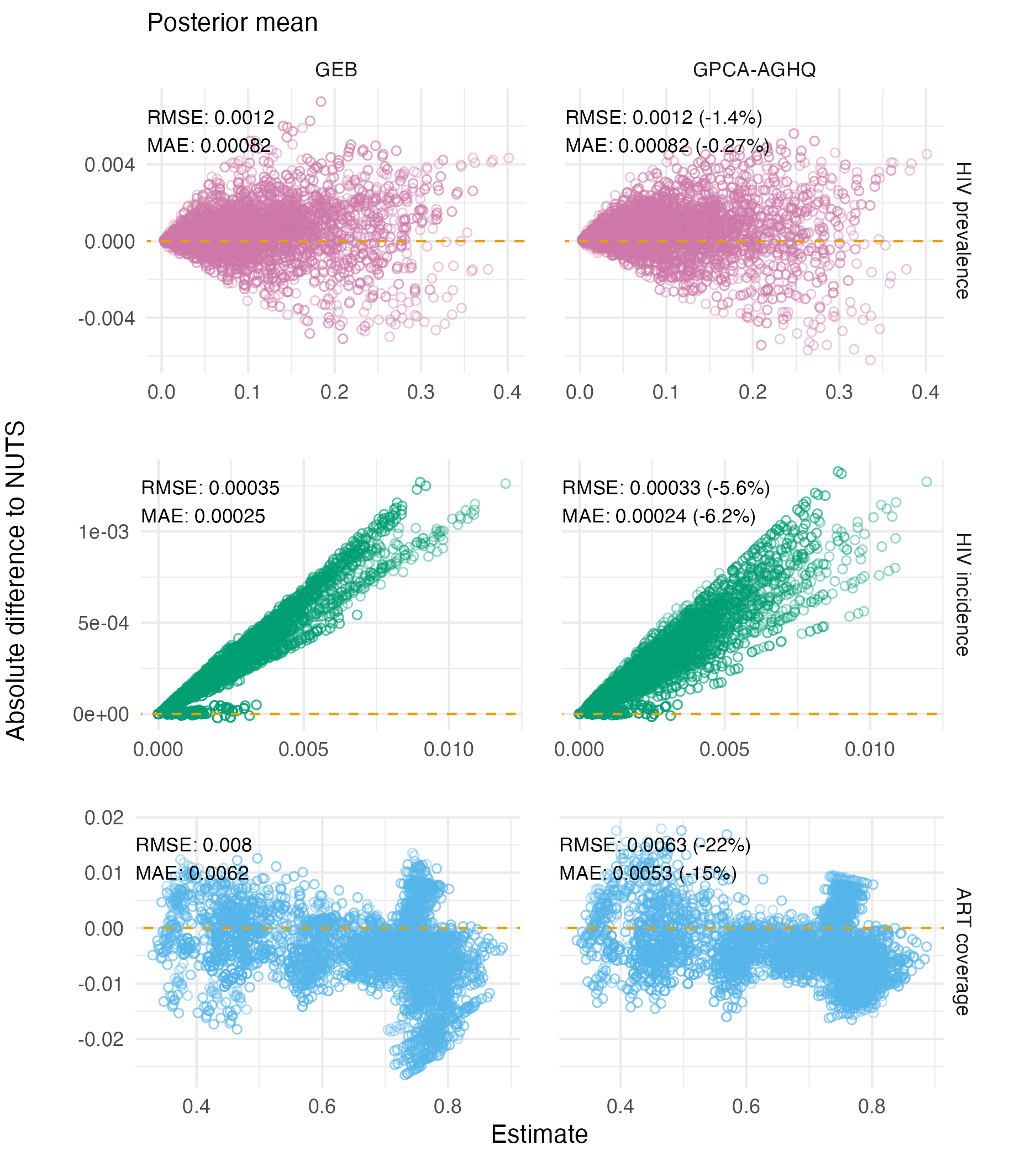
Figure C.15: Differences in Naomi model output posterior means as estimated by GEB and GPCA-AGHQ compared to NUTS. Each point is an estimate of the indicator for a particular strata. In all cases, error is reduced by GPCA-AGHQ, most of all for ART coverage.

Differences in Naomi model output posterior standard deviations as estimated by GEB and GPCA-AGHQ compared to NUTS. Each point is an estimate of the indicator for a particular strata. Error is increased by GPCA-AGHQ for HIV prevalence and HIV indicdence, and reduced for ART coverage.

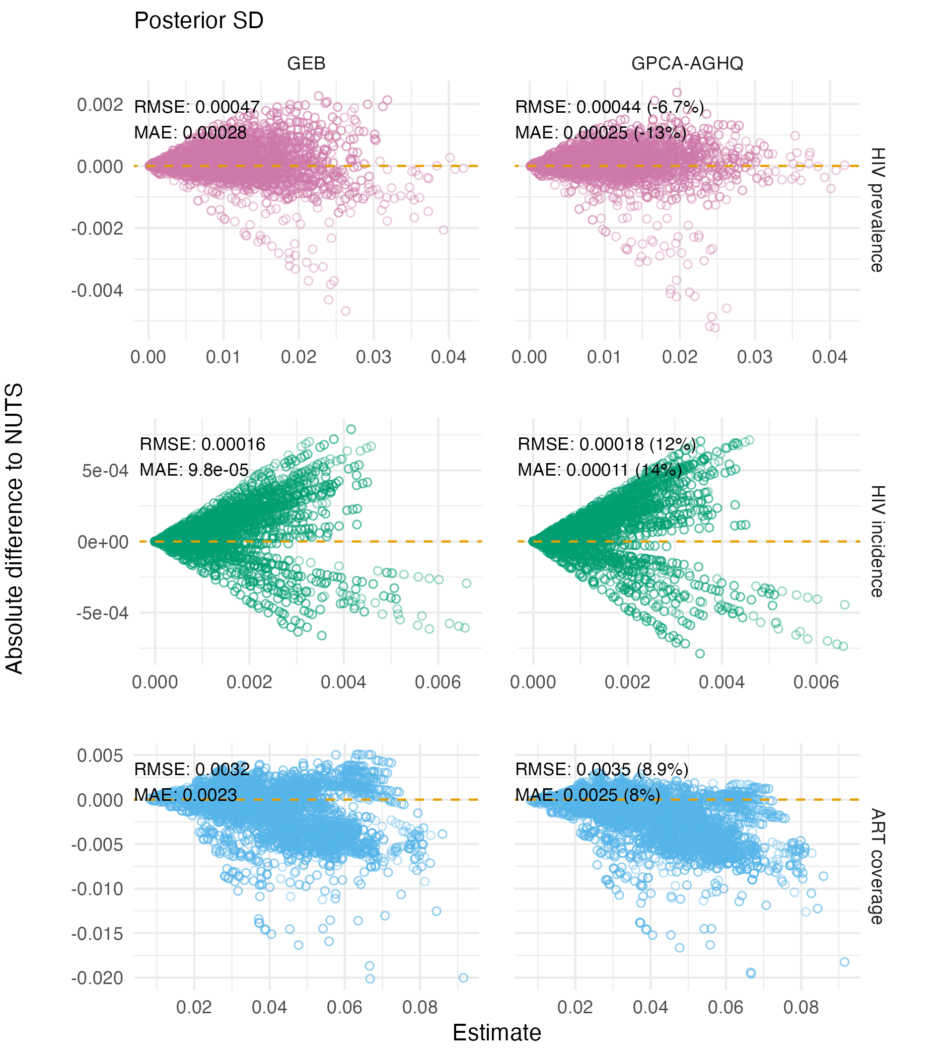
Figure C.16: Differences in Naomi model output posterior standard deviations as estimated by GEB and GPCA-AGHQ compared to NUTS. Each point is an estimate of the indicator for a particular strata. Error is increased by GPCA-AGHQ for HIV prevalence and HIV indicdence, and reduced for ART coverage.

C.7.2 Distributional quantities
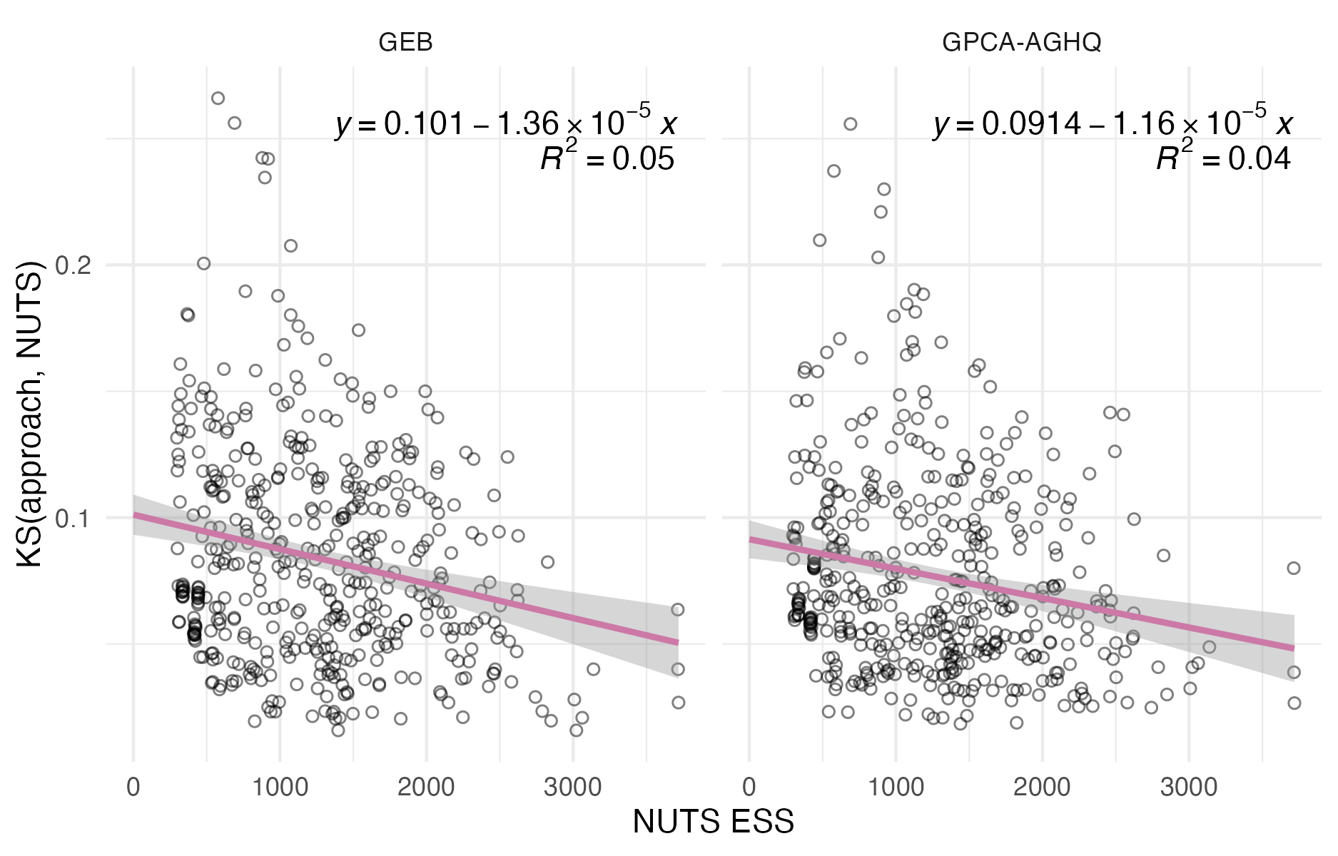
The Kolomogorov-Smirnov (KS) test statistic for each latent field parameter is correlated with the effective sample size (ESS) from NUTS, for both GEB and GPCA-AGHQ. This may be because parameters which are harder to estimate with INLA-like methods also have posterior distributions which are more difficult to sample from. Alternatively, it may be that high KS values are caused by inaccurate NUTS estimates generated by limited effective samples.

Figure C.17: The Kolomogorov-Smirnov (KS) test statistic for each latent field parameter is correlated with the effective sample size (ESS) from NUTS, for both GEB and GPCA-AGHQ. This may be because parameters which are harder to estimate with INLA-like methods also have posterior distributions which are more difficult to sample from. Alternatively, it may be that high KS values are caused by inaccurate NUTS estimates generated by limited effective samples.

Akaike, Hirotugu. 1973. Information theory as an extension of the maximum likelihood principle–In: Second International Symposium on Information Theory (Eds) BN Petrov, F.” Csaki. BNPBF Csaki Budapest: Academiai Kiado.
Aldor-Noiman, Sivan, Lawrence D Brown, Andreas Buja, Wolfgang Rolke, and Robert A Stine. 2013. The power to see: A new graphical test of normality.” The American Statistician 67 (4): 249–60.
Arambepola, Rohan, Tim CD Lucas, Anita K Nandi, Peter W Gething, and Ewan Cameron. 2022. A simulation study of disaggregation regression for spatial disease mapping.” Statistics in Medicine 41 (1): 1–16.
Auvert, Bertran, Dirk Taljaard, Emmanuel Lagarde, Joelle Sobngwi-Tambekou, Rémi Sitta, and Adrian Puren. 2005. Randomized, controlled intervention trial of male circumcision for reduction of HIV infection risk: the ANRS 1265 Trial.” PLoS Medicine 2 (11): e298.
Bachl, Fabian E, Finn Lindgren, David L Borchers, and Janine B Illian. 2019. inlabru: an R package for Bayesian spatial modelling from ecological survey data.” Methods in Ecology and Evolution 10 (6): 760–66.
Baeten, Jared M, Deborah Donnell, Patrick Ndase, Nelly R Mugo, James D Campbell, Jonathan Wangisi, Jordan W Tappero, et al. 2012. “Antiretroviral Prophylaxis for HIV Prevention in Heterosexual Men and Women.” New England Journal of Medicine 367 (5): 399–410.
Bailey, Michael A. 2023. “A New Paradigm for Polling.” Harvard Data Science Review 5 (3).
Bailey, Robert C, Stephen Moses, Corette B Parker, Kawango Agot, Ian Maclean, John N Krieger, Carolyn FM Williams, Richard T Campbell, and Jeckoniah O Ndinya-Achola. 2007. Male circumcision for HIV prevention in young men in Kisumu, Kenya: a randomised controlled trial.” The Lancet 369 (9562): 643–56.
Baker, Stuart G. 1994. The multinomial-Poisson transformation.” Journal of the Royal Statistical Society: Series D (The Statistician) 43 (4): 495–504.
Baral, Stefan, Chris Beyrer, Kathryn Muessig, Tonia Poteat, Andrea L Wirtz, Michele R Decker, Susan G Sherman, and Deanna Kerrigan. 2012. Burden of HIV among female sex workers in low-income and middle-income countries: a systematic review and meta-analysis.” The Lancet Infectious Diseases 12 (7): 538–49.
Barré-Sinoussi, Françoise, Jean-Claude Chermann, Fran Rey, Marie Therese Nugeyre, Sophie Chamaret, Jacqueline Gruest, Charles Dauguet, et al. 1983. Isolation of a T-lymphotropic retrovirus from a patient at risk for acquired immune deficiency syndrome (AIDS).” Science 220 (4599): 868–71.
Baydin, Atılım Günes, Barak A Pearlmutter, Alexey Andreyevich Radul, and Jeffrey Mark Siskind. 2017. Automatic differentiation in machine learning: a survey.” The Journal of Machine Learning Research 18 (1): 5595–5637.
Bell, Bradley. 2023. CppAD: a package for C++ algorithmic differentiation.” http://www.coin-or.org/CppAD.
Bennett, James E, Helen Tamura-Wicks, Robbie M Parks, Richard T Burnett, C Arden Pope III, Matthew J Bechle, Julian D Marshall, Goodarz Danaei, and Majid Ezzati. 2019. Particulate matter air pollution and national and county life expectancy loss in the USA: A spatiotemporal analysis.” PLoS Medicine 16 (7): e1002856.
Berger, James. 2006. The Case for objective Bayesian analysis.” Bayesian Analysis 1 (3): 385–402.
Berild, Martin Outzen, Sara Martino, Virgilio Gómez-Rubio, and Håvard Rue. 2022. “Importance Sampling with the Integrated Nested Laplace Approximation.” Journal of Computational and Graphical Statistics 31 (4): 1225–37.
Bernardo, José M, and Adrian FM Smith. 2001. Bayesian theory. John Wiley & Sons.
Besag, Julian, Jeremy York, and Annie Mollié. 1991. Bayesian image restoration, with two applications in spatial statistics.” Annals of the Institute of Statistical Mathematics 43 (1): 1–20.
Best, N, N Arnold, A Thomas, L Waller, and E Conlon. 1999. Bayesian models for spatially correlated disease and exposure data.” In Bayesian Statistics 6: Proceedings of the Sixth Valencia International Meeting, 6:131. Oxford University Press.
Best, Nicky, Sylvia Richardson, and Andrew Thomson. 2005. A comparison of Bayesian spatial models for disease mapping.” Statistical Methods in Medical Research 14 (1): 35–59.
Betancourt, Michael. 2017. Robust Gaussian processes in Stan.” https://betanalpha.github.io/assets/case\%5Fstudies/gp\%5Fpart3/part3.html.
Bhatt, Samir, DJ Weiss, E Cameron, D Bisanzio, B Mappin, U Dalrymple, KE Battle, et al. 2015. The effect of malaria control on Plasmodium falciparum in Africa between 2000 and 2015.” Nature 526 (7572): 207–11.
Bilodeau, Blair, Alex Stringer, and Yanbo Tang. 2022. Stochastic convergence rates and applications of adaptive quadrature in Bayesian inference.” Journal of the American Statistical Association, 1–11.
Bivand, Roger S, Edzer J Pebesma, Virgilio Gómez-Rubio, and Edzer Jan Pebesma. 2008. Applied spatial data analysis with R. Springer.
Blangiardo, Marta, Michela Cameletti, Gianluca Baio, and Håvard Rue. 2013. Spatial and spatio-temporal models with R-INLA.” Spatial and Spatio-Temporal Epidemiology 4: 33–49.
Blei, David M, Alp Kucukelbir, and Jon D McAuliffe. 2017. Variational inference: A review for statisticians.” Journal of the American Statistical Association 112 (518): 859–77.
Bolker, Benjamin M, Beth Gardner, Mark Maunder, Casper W Berg, Mollie Brooks, Liza Comita, Elizabeth Crone, et al. 2013. Strategies for fitting nonlinear ecological models in R, AD Model Builder, and BUGS.” Methods in Ecology and Evolution 4 (6): 501–12.
Bollhöfer, Matthias, Olaf Schenk, Radim Janalik, Steve Hamm, and Kiran Gullapalli. 2020. State-of-the-art sparse direct solvers.” Parallel Algorithms in Computational Science and Engineering, 3–33.
Bosse, Nikos I, Sam Abbott, Anne Cori, Edwin van Leeuwen, Johannes Bracher, and Sebastian Funk. 2023. Scoring epidemiological forecasts on transformed scales.” PLoS Computational Biology 19 (8): e1011393.
Bosse, Nikos I., Hugo Gruson, Anne Cori, Edwin van Leeuwen, Sebastian Funk, and Sam Abbott. 2022. Evaluating Forecasts with scoringutils in R.” arXiv. https://arxiv.org/abs/2205.07090.
Box, George EP, and Kenneth B Wilson. 1992. On the experimental attainment of optimum conditions.” In Breakthroughs in Statistics: Methodology and Distribution, 270–310. Springer.
Bradley, Valerie C, Shiro Kuriwaki, Michael Isakov, Dino Sejdinovic, Xiao-Li Meng, and Seth Flaxman. 2021. “Unrepresentative Big Surveys Significantly Overestimated US Vaccine Uptake.” Nature 600 (7890): 695–700.
Breslow, Norman E, and David G Clayton. 1993. Approximate inference in generalized linear mixed models.” Journal of the American Statistical Association 88 (421): 9–25.
Brier, Glenn W. 1950. Verification of forecasts expressed in terms of probability.” Monthly Weather Review 78 (1): 1–3.
Brooks, Mollie E, Kasper Kristensen, Koen J Van Benthem, Arni Magnusson, Casper W Berg, Anders Nielsen, Hans J Skaug, Martin Machler, and Benjamin M Bolker. 2017. glmmTMB balances speed and flexibility among packages for zero-inflated generalized linear mixed modeling.” The R Journal 9 (2): 378–400.
Brown, Patrick E. 2015. Model-based geostatistics the easy way.” Journal of Statistical Software 63: 1–24.
Broyles, Laura N, Robert Luo, Debi Boeras, and Lara Vojnov. 2023. The risk of sexual transmission of HIV in individuals with low-level HIV viraemia: a systematic review.” The Lancet.
Brugh, Kristen N, Quinn Lewis, Cameron Haddad, Jon Kumaresan, Timothy Essam, and Michelle S Li. 2021. Characterizing and mapping the spatial variability of HIV risk among adolescent girls and young women: A cross-county analysis of population-based surveys in Eswatini, Haiti, and Mozambique.” PLoS One 16 (12): e0261520.
Bürkner, Paul-Christian. 2017. brms: An R Package for Bayesian Multilevel Models Using Stan.” Journal of Statistical Software 80 (1): 1–28. https://doi.org/10.18637/jss.v080.i01.
Carpenter, Bob, Andrew Gelman, Matthew D Hoffman, Daniel Lee, Ben Goodrich, Michael Betancourt, Marcus Brubaker, Jiqiang Guo, Peter Li, and Allen Riddell. 2017. Stan: A probabilistic programming language.” Journal of Statistical Software 76 (1).
Casella, George. 1985. An introduction to empirical Bayes data analysis.” The American Statistician 39 (2): 83–87.
CDC. 2014. “Understanding the HIV Care Continuum.” CDC. http://www.cdc.gov/hiv/pdf/dhap_continuum.pdf.
Chau, Siu Lun, Shahine Bouabid, and Dino Sejdinovic. 2021. Deconditional downscaling with Gaussian processes.” Advances in Neural Information Processing Systems 34: 17813–25.
Chen, Cici, Jon Wakefield, and Thomas Lumely. 2014. The use of sampling weights in Bayesian hierarchical models for small area estimation.” Spatial and Spatio-Temporal Epidemiology 11: 33–43.
Chopin, Nicolas, Omiros Papaspiliopoulos, et al. 2020. An introduction to sequential Monte Carlo. Vol. 4. Springer.
Cleland, John, J Ties Boerma, Michel Caraël, and Sharon S Weir. 2004. Monitoring sexual behaviour in general populations: a synthesis of lessons of the past decade.” Sexually Transmitted Infections 80 (suppl 2): ii1–7.
Cohen, Myron S, Ying Q Chen, Marybeth McCauley, Theresa Gamble, Mina C Hosseinipour, Nagalingeswaran Kumarasamy, James G Hakim, et al. 2011. Prevention of HIV-1 infection with early antiretroviral therapy.” New England Journal of Medicine 365 (6): 493–505.
Cramb, SM, EW Duncan, PD Baade, and KL Mengersen. 2018. Investigation of Bayesian spatial models.” Cancer Council Queensland; Queensland University of Technology (QUT).
Crampin, Amelia C, Albert Dube, Sebastian Mboma, Alison Price, Menard Chihana, Andreas Jahn, Angela Baschieri, et al. 2012. Profile: the Karonga health and demographic surveillance system.” International Journal of Epidemiology 41 (3): 676–85.
Cressie, Noel, and Christopher K Wikle. 2015. Statistics for spatio-temporal data. John Wiley & Sons.
Csárdi, Gábor. 2023. cranlogs: Download Logs from the ’RStudio’ ’CRAN’ Mirror.
Davis, Philip J, and Philip Rabinowitz. 1975. Methods of numerical integration. Academic Press.
Dawid, A Philip. 1984. Present position and potential developments: Some personal views statistical theory the prequential approach.” Journal of the Royal Statistical Society: Series A (General) 147 (2): 278–90.
de Valpine, Perry, Christopher Paciorek, Daniel Turek, Nick Michaud, Cliff Anderson-Bergman, Fritz Obermeyer, Claudia Wehrhahn Cortes, Abel Rodrìguez, Duncan Temple Lang, and Sally Paganin. 2023. NIMBLE User Manual (version 1.0.1). https://doi.org/10.5281/zenodo.1211190.
Dean, CB, MD Ugarte, and AF Militino. 2001. Detecting interaction between random region and fixed age effects in disease mapping.” Biometrics 57 (1): 197–202.
Dempster, Arthur P, Nan M Laird, and Donald B Rubin. 1977. Maximum likelihood from incomplete data via the EM algorithm.” Journal of the Royal Statistical Society: Series B (Methodological) 39 (1): 1–22.
Dennis Jr, John E, David M Gay, and Roy E Walsh. 1981. An adaptive nonlinear least-squares algorithm.” ACM Transactions on Mathematical Software (TOMS) 7 (3): 348–68.
Diaz, Jose Monsalve, Swaroop Pophale, Oscar Hernandez, David E Bernholdt, and Sunita Chandrasekaran. 2018. OpenMP 4.5 Validation and Verification Suite for Device Offload.” In Evolving OpenMP for Evolving Architectures: 14th International Workshop on OpenMP, IWOMP 2018, Barcelona, Spain, September 26–28, 2018, Proceedings 14, 82–95. Springer.
Diggle, Peter J, and Emanuele Giorgi. 2016. Model-based geostatistics for prevalence mapping in low-resource settings.” Journal of the American Statistical Association 111 (515): 1096–1120.
Diggle, Peter J, Paula Moraga, Barry Rowlingson, Benjamin M Taylor, et al. 2013. Spatial and spatio-temporal log-Gaussian Cox processes: extending the geostatistical paradigm.” Statistical Science 28 (4): 542–63.
Dominguez, Kenneth L., Dawn K. Smith, Vasavi Thomas, Nicole Crepaz, Karen Lang, Walid Heneine, Janet M. McNicholl, et al. 2016. “Updated Guidelines for Antiretroviral Postexposure Prophylaxis After Sexual, Injection Drug Use, or Other Nonoccupational Exposure to HIV—United States, 2016.” https://stacks.cdc.gov/view/cdc/38856.
Donegan, Connor. 2022. geostan: An R package for Bayesian spatial analysis.” The Journal of Open Source Software 7 (79): 4716. https://doi.org/10.21105/joss.04716.
Duane, Simon, Anthony D Kennedy, Brian J Pendleton, and Duncan Roweth. 1987. Hybrid Monte Carlo.” Physics Letters B 195 (2): 216–22.
Duncan, Earl W, Nicole M White, and Kerrie Mengersen. 2017. Spatial smoothing in Bayesian models: a comparison of weights matrix specifications and their impact on inference.” International Journal of Health Geographics 16 (1): 1–16.
Dwyer-Lindgren, Laura, Michael A Cork, Amber Sligar, Krista M Steuben, Kate F Wilson, Naomi R Provost, Benjamin K Mayala, et al. 2019. Mapping HIV prevalence in sub-Saharan Africa between 2000 and 2017.” Nature 570 (7760): 189–93.
Dwyer-Lindgren, Laura, Abraham D Flaxman, Marie Ng, Gillian M Hansen, Christopher JL Murray, and Ali H Mokdad. 2015. Drinking patterns in US counties from 2002 to 2012.” American Journal of Public Health 105 (6): 1120–27.
Eaton, Jeffrey W, Laura Dwyer-Lindgren, Steve Gutreuter, Megan O’Driscoll, Oliver Stevens, Sumali Bajaj, Rob Ashton, et al. 2021. Naomi: a new modelling tool for estimating HIV epidemic indicators at the district level in sub-Saharan Africa.” Journal of the International AIDS Society 24: e25788.
Economist Impact. 2023. A triple dividend: the health, social and economic gains from financing the HIV response in Africa.”
Esra, Rachel, Mpho Mmelesi, Akeem T. Ketlogetswe, Timothy M. Wolock, Adam Howes, Tlotlo Nong, Matshelo Tina Matlhaga, Siphiwe Ratladi, Dinah Ramaabya, and Jeffrey W. Imai-Eaton. 2024. “Improved Indicators for Subnational Unmet Antiretroviral Therapy Need in the Health System: Updates to the Naomi Model in 2023.” JAIDS Journal of Acquired Immune Deficiency Syndromes 95 (1S): e24–33. https://doi.org/10.1097/QAI.0000000000003324.
Fattah, EA, JV Niekerk, and H Rue. 2022. Smart gradient-an adaptive technique for improving gradient estimation.” Foundations of Data Science.
Fay, Robert E, and Roger A Herriot. 1979. Estimates of income for small places: an application of James-Stein procedures to census data.” Journal of the American Statistical Association 74 (366a): 269–77.
Fisher, Ronald Aylmer. 1936. Design of experiments.” British Medical Journal 1 (3923): 554.
FitzJohn, Rich, Robert Ashton, Alex Hill, Martin Eden, Wes Hinsley, Emma Russell, and James Thompson. 2023. Orderly: Lightweight Reproducible Reporting.
Flaxman, Seth R, Yu-Xiang Wang, and Alexander J Smola. 2015. Who supported Obama in 2012? Ecological inference through distribution regression.” In Proceedings of the 21th ACM SIGKDD International Conference on Knowledge Discovery and Data Mining, 289–98.
Follestad, Turid, and Håvard Rue. 2003. Modelling spatial variation in disease risk using Gaussian Markov random field proxies for Gaussian random fields.”
Fournier, David A, Hans J Skaug, Johnoel Ancheta, James Ianelli, Arni Magnusson, Mark N Maunder, Anders Nielsen, and John Sibert. 2012. AD Model Builder: using automatic differentiation for statistical inference of highly parameterized complex nonlinear models.” Optimization Methods and Software 27 (2): 233–49.
Freni-Sterrantino, Anna, Massimo Ventrucci, and Håvard Rue. 2018. A note on intrinsic conditional autoregressive models for disconnected graphs.” Spatial and Spatio-Temporal Epidemiology 26: 25–34.
Fuglstad, Geir-Arne, Daniel Simpson, Finn Lindgren, and Håvard Rue. 2019. Constructing priors that penalize the complexity of Gaussian random fields.” Journal of the American Statistical Association 114 (525): 445–52.
Gaedke-Merzhäuser, Lisa, Janet van Niekerk, Olaf Schenk, and Håvard Rue. 2023. Parallelized integrated nested Laplace approximations for fast Bayesian inference.” Statistics and Computing 33 (1): 25.
Garnier, Simon, Ross, Noam, Rudis, Robert, Camargo, et al. 2023. viridis(Lite) - Colorblind-Friendly Color Maps for R. https://doi.org/10.5281/zenodo.4679423.
Gärtner, Thomas, Peter A Flach, Adam Kowalczyk, and Alexander J Smola. 2002. Multi-instance kernels.” In ICML, 2:7. 3.
Gelfand, Alan E, Li Zhu, and Bradley P Carlin. 2001. On the change of support problem for spatio-temporal data.” Biostatistics 2 (1): 31–45.
Gelman, Andrew. 2005. Analysis of variance—why it is more important than ever.”
———. 2006. Prior distributions for variance parameters in hierarchical models (comment on article by Browne and Draper).” Bayesian Analysis 1 (3): 515–34.
———. 2007. Struggles with survey weighting and regression modeling.”
Gelman, Andrew, John B Carlin, Hal S Stern, David B Dunson, Aki Vehtari, and Donald B Rubin. 2013. Bayesian data analysis. CRC press.
Gelman, Andrew, Jessica Hwang, and Aki Vehtari. 2014. Understanding predictive information criteria for Bayesian models.” Statistics and Computing 24 (6): 997–1016.
Gelman, Andrew, and Donald B Rubin. 1992. Inference from iterative simulation using multiple sequences.” Statistical Science, 457–72.
Gelman, Andrew, Daniel Simpson, and Michael Betancourt. 2017. The prior can often only be understood in the context of the likelihood.” Entropy 19 (10): 555.
Gelman, Andrew, Aki Vehtari, Daniel Simpson, Charles C Margossian, Bob Carpenter, Yuling Yao, Lauren Kennedy, Jonah Gabry, Paul-Christian Bürkner, and Martin Modrák. 2020. Bayesian workflow.” arXiv Preprint arXiv:2011.01808.
Geman, Stuart, and Donald Geman. 1984. Stochastic relaxation, Gibbs distributions, and the Bayesian restoration of images.” IEEE Transactions on Pattern Analysis and Machine Intelligence, no. 6: 721–41.
Giordano, Ryan, Tamara Broderick, and Michael I. Jordan. 2018. Covariances, Robustness, and Variational Bayes.” Journal of Machine Learning Research 19 (51): 1–49. http://jmlr.org/papers/v19/17-670.html.
Global Burden of Disease Collaborative Network. 2019. Global Burden of Disease Study 2019 (GBD 2019) Results. Institute for Health Metrics and Evaluation (IHME). https://vizhub.healthdata.org/gbd-results/.
Glynn, Judith R, Ndoliwe Kayuni, Emmanuel Banda, Fiona Parrott, Sian Floyd, Monica Francis-Chizororo, Misheck Nkhata, et al. 2011. Assessing the validity of sexual behaviour reports in a whole population survey in rural Malawi.” PLoS One 6 (7): e22840.
Gneiting, Tilmann, and Adrian E Raftery. 2007. Strictly proper scoring rules, prediction, and estimation.” Journal of the American Statistical Association 102 (477): 359–78.
Godfrey-Faussett, Peter, Luisa Frescura, Quarraisha Abdool Karim, Michaela Clayton, Peter D Ghys, and 2025 prevention targets working group). 2022. “HIV Prevention for the Next Decade: Appropriate, Person-Centred, Prioritised, Effective, Combination Prevention.” PLoS Medicine 19 (9): e1004102.
Goldstein, Michael. 2006. Subjective Bayesian analysis: principles and practice.”
Gómez-Rubio, Virgilio. 2020. Bayesian inference with INLA. CRC Press.
Gómez-Rubio, Virgilio, and Håvard Rue. 2018. “Markov Chain Monte Carlo with the Integrated Nested Laplace Approximation.” Statistics and Computing 28: 1033–51.
Goodrich, Ben, Jonah Gabry, Imad Ali, and Sam Brilleman. 2020. “Rstanarm: Bayesian Applied Regression Modeling via Stan.” https://mc-stan.org/rstanarm.
Gössl, Christoff, Dorothee P Auer, and Ludwig Fahrmeir. 2001. Bayesian spatiotemporal inference in functional magnetic resonance imaging.” Biometrics 57 (2): 554–62.
Gottlieb, Michael S, Howard M Schanker, Peng Thim Fan, Andrew Saxon, Joel D Weisman, Irving Pozalski, et al. 1981. Pneumocystis pneumonia—Los Angeles.” Morbidity and Mortality Weekly Report 30 (21): 1–3.
Grabowski, M Kate, David M Serwadda, Ronald H Gray, Gertrude Nakigozi, Godfrey Kigozi, Joseph Kagaayi, Robert Ssekubugu, et al. 2017. HIV prevention efforts and incidence of HIV in Uganda.” New England Journal of Medicine 377 (22): 2154–66.
Gray, Ronald H, Godfrey Kigozi, David Serwadda, Frederick Makumbi, Stephen Watya, Fred Nalugoda, Noah Kiwanuka, et al. 2007. Male circumcision for HIV prevention in men in Rakai, Uganda: a randomised trial.” The Lancet 369 (9562): 657–66.
Gregson, Simon, Geoffrey P Garnett, Constance A Nyamukapa, Timothy B Hallett, James JC Lewis, Peter R Mason, Stephen K Chandiwana, and Roy M Anderson. 2006. HIV decline associated with behavior change in eastern Zimbabwe.” Science 311 (5761): 664–66.
Gretton, Arthur, Karsten Borgwardt, Malte Rasch, Bernhard Schölkopf, and Alex Smola. 2006. “A Kernel Method for the Two-Sample-Problem.” Advances in Neural Information Processing Systems 19.
Grieve, Richard, Youqi Yang, Sam Abbott, Giridhara R Babu, Malay Bhattacharyya, Natalie Dean, Stephen Evans, et al. 2023. “The Importance of Investing in Data, Models, Experiments, Team Science, and Public Trust to Help Policymakers Prepare for the Next Pandemic.” PLOS Global Public Health 3 (11): e0002601.
Haining, Robert P. 2003. Spatial data analysis: theory and practice. Cambridge University Press.
Hájek, Jaroslav. 1971. Discussion of ‘An essay on the logical foundations of survey sampling, part I’.” Foundations of Statistical Inference (Proc. Sympos., Univ. Waterloo, Ontario, 1970), 236.
Hamelijnck, O, T Damoulas, K Wang, and MA Girolami. 2019. Multi-resolution multi-task Gaussian processes.” Advances in Neural Information Processing Systems 32.
Hastie, Trevor, and Robert Tibshirani. 1987. Generalized additive models: some applications.” Journal of the American Statistical Association 82 (398): 371–86.
Hastings, W. K. 1970. “Monte Carlo Sampling Methods Using Markov Chains and Their Applications.” Biometrika 57 (1): 97–109. http://www.jstor.org/stable/2334940.
Helleringer, Stéphane, Hans-Peter Kohler, Linda Kalilani-Phiri, James Mkandawire, and Benjamin Armbruster. 2011. The reliability of sexual partnership histories: implications for the measurement of partnership concurrency during surveys.” AIDS (London, England) 25 (4): 503.
Hodgins, Caroline, James Stannah, Salome Kuchukhidze, Lycias Zembe, Jeffrey W Eaton, Marie-Claude Boily, and Mathieu Maheu-Giroux. 2022. Population sizes, HIV prevalence, and HIV prevention among men who paid for sex in sub-Saharan Africa (2000–2020): A meta-analysis of 87 population-based surveys.” PLoS Medicine 19 (1): e1003861.
Hoffman, Matthew D, Andrew Gelman, et al. 2014. The No-U-Turn sampler: adaptively setting path lengths in Hamiltonian Monte Carlo. J. Mach. Learn. Res. 15 (1): 1593–623.
Howes, Adam. 2023a. arealutils: Utility functions for beyond-borders.
———. 2023b. multi.utils: Utility functions for multi-agyw.
Howes, Adam, Kathryn A. Risher, Van Kính Nguyen, Oliver Stevens, Katherine M. Jia, Timothy M. Wolock, Rachel T. Esra, et al. 2023. Spatio-temporal estimates of HIV risk group proportions for adolescent girls and young women across 13 priority countries in sub-Saharan Africa.” PLOS Global Public Health 3 (4): 1–14. https://doi.org/10.1371/journal.pgph.0001731.
ICAP. 2023. Population-based HIV impact assessment: guiding the global HIV response.” https://phia.icap.columbia.edu.
Jäckel, Peter. 2005. A note on multivariate Gauss-Hermite quadrature.” London: ABN-Amro. Re.
Jia, Katherine M, Hallie Eilerts, Olanrewaju Edun, Kevin Lam, Adam Howes, Matthew L Thomas, and Jeffrey W Eaton. 2022. Risk scores for predicting HIV incidence among adult heterosexual populations in sub-Saharan Africa: a systematic review and meta-analysis.” Journal of the International AIDS Society 25 (1): e25861.
Jin, Harry, Arjee Restar, and Chris Beyrer. 2021. “Overview of the Epidemiological Conditions of HIV Among Key Populations in Africa.” Journal of the International AIDS Society 24: e25716.
Johnson, L, and RE Dorrington. 2020. Thembisa version 4.3: A model for evaluating the impact of HIV/AIDS in South Africa.” View Article.
Johnson, Olatunji, Peter Diggle, and Emanuele Giorgi. 2019. A spatially discrete approximation to log-Gaussian Cox processes for modelling aggregated disease count data.” Statistics in Medicine 38 (24): 4871–87.
Karatzoglou, Alexandros, Alex Smola, Kurt Hornik, and Maintainer Alexandros Karatzoglou. 2019. “Package ‘Kernlab’.” CRAN R Project.
Kassanjee, Reshma, Thomas A. McWalter, Till Bärnighausen, and Alex Welte. 2012. “A New General Biomarker-Based Incidence Estimator.” Epidemiology 23 (5).
Kelsall, Julia, and Jonathan Wakefield. 2002. Modeling spatial variation in disease risk: a geostatistical approach.” Journal of the American Statistical Association 97 (459): 692–701.
Khoury, Muin J, Michael F Iademarco, and William T Riley. 2016. Precision public health for the era of precision medicine.” American Journal of Preventive Medicine 50 (3): 398–401.
Kish, Leslie. 1965. Survey sampling. 04; HN29, K5.
Knorr-Held, Leonhard. 2000. Bayesian modelling of inseparable space-time variation in disease risk.” Statistics in Medicine 19 (17-18): 2555–67.
Konstantinoudis, Garyfallos, Dominic Schuhmacher, Håvard Rue, and Ben D Spycher. 2020. Discrete versus continuous domain models for disease mapping.” Spatial and Spatio-Temporal Epidemiology 32: 100319.
Kristensen, Kasper. 2021. The comprehensive TMB documentation.” https://kaskr.github.io/adcomp/_book/Introduction.html.
Kristensen, Kasper, Anders Nielsen, Casper W Berg, Hans Skaug, Bradley M Bell, et al. 2016. TMB: Automatic Differentiation and Laplace Approximation.” Journal of Statistical Software 70 (i05).
Laplace, P. S. 1774. Memoire sur la probabilite de causes par les evenements.” Memoire de l’Academie Royale Des Sciences.
Law, Ho Chung, Dino Sejdinovic, Ewan Cameron, Tim Lucas, Seth Flaxman, Katherine Battle, and Kenji Fukumizu. 2018. Variational learning on aggregate outputs with Gaussian processes.” Advances in Neural Information Processing Systems 31.
Lee, Duncan. 2011. A comparison of conditional autoregressive models used in Bayesian disease mapping.” Spatial and Spatio-Temporal Epidemiology 2 (2): 79–89.
Lenth, Russell. 2009. Response-Surface Methods in R, Using rsm.” Journal of Statistical Software 32 (7): 1–17. https://doi.org/10.18637/jss.v032.i07.
Leppik, IE, FE Dreifuss, T Bowman-Cloyd, N Santilli, M Jacobs, C Crosby, J Cloyd, et al. 1985. A double-blind crossover evaluation of progabide in partial seizures.” Neurology 35 (4): 285.
Leroux, Brian G, Xingye Lei, and Norman Breslow. 2000. Estimation of disease rates in small areas: a new mixed model for spatial dependence.” In Statistical Models in Epidemiology, the Environment, and Clinical Trials, 179–91. Springer.
Li, Ye, Patrick Brown, Dionne C Gesink, and Håvard Rue. 2012. Log Gaussian Cox processes and spatially aggregated disease incidence data.” Statistical Methods in Medical Research 21 (5): 479–507. https://doi.org/10.1177/0962280212446326.
Lindgren, Finn, Håvard Rue, and Johan Lindström. 2011. An explicit link between Gaussian fields and Gaussian Markov random fields: the stochastic partial differential equation approach.” Journal of the Royal Statistical Society Series B: Statistical Methodology 73 (4): 423–98.
Margossian, Charles C. 2019. A review of automatic differentiation and its efficient implementation.” Wiley Interdisciplinary Reviews: Data Mining and Knowledge Discovery 9 (4): e1305.
Margossian, Charles C, and Andrew Gelman. 2023. “For How Many Iterations Should We Run Markov Chain Monte Carlo?” arXiv Preprint arXiv:2311.02726.
Margossian, Charles, Aki Vehtari, Daniel Simpson, and Raj Agrawal. 2020. Hamiltonian Monte Carlo using an adjoint-differentiated Laplace approximation: Bayesian inference for latent Gaussian models and beyond.” Advances in Neural Information Processing Systems 33: 9086–97.
Martin, Gael M, David T Frazier, and Christian P Robert. 2023. Computing Bayes: From then ‘til now.” Statistical Science 1 (1): 1–17.
Martino, Sara, and Andrea Riebler. 2020. Integrated Nested Laplace Approximations (INLA).” In Wiley StatsRef: Statistics Reference Online, 1–19. John Wiley & Sons, Ltd. https://doi.org/https://doi.org/10.1002/9781118445112.stat08212.
Martino, Sara, and Håvard Rue. 2009. Implementing approximate Bayesian inference using Integrated Nested Laplace Approximation: A manual for the inla program.” Department of Mathematical Sciences, NTNU, Norway.
Martins, Thiago G, Daniel Simpson, Finn Lindgren, and Håvard Rue. 2013. Bayesian computing with INLA: new features.” Computational Statistics & Data Analysis 67: 68–83.
Matheson, James E, and Robert L Winkler. 1976. Scoring rules for continuous probability distributions.” Management Science 22 (10): 1087–96.
Mayala, Benjamin K., Samir Bhatt, and Peter Gething. 2020. Predicting HIV/AIDS at Subnational Levels using DHS Covariates related to HIV.” DHS Spatial Analysis Reports 18. Rockville, Maryland, USA: ICF.
McCullagh, Peter, and John A Nelder. 1989. Generalized linear models. Routledge.
McElreath, Richard. 2020. Statistical rethinking: A Bayesian course with examples in R and Stan. CRC press.
McGillen, Jessica B, John Stover, Daniel J Klein, Sinokuthemba Xaba, Getrude Ncube, Mutsa Mhangara, Geraldine N Chipendo, et al. 2018. “The Emerging Health Impact of Voluntary Medical Male Circumcision in Zimbabwe: An Evaluation Using Three Epidemiological Models.” PloS One 13 (7): e0199453.
Meng, Xiao-Li. 2018. Statistical paradises and paradoxes in big data (i) law of large populations, big data paradox, and the 2016 US presidential election.” The Annals of Applied Statistics 12 (2): 685–726.
Metropolis, Nicholas, Arianna W Rosenbluth, Marshall N Rosenbluth, Augusta H Teller, and Edward Teller. 1953. Equation of State Calculations by Fast Computing Machines.” J. Chem. Phys 21: 1087.
Meyer-Rath, Gesine, Jessica B McGillen, Diego F Cuadros, Timothy B Hallett, Samir Bhatt, Njeri Wabiri, Frank Tanser, and Thomas Rehle. 2018. “Targeting the Right Interventions to the Right People and Places: The Role of Geospatial Analysis in HIV Program Planning.” AIDS (London, England) 32 (8): 957.
Minka, Thomas P. 2001. Expectation Propagation for approximate Bayesian inference.” In Proceedings of the 17th Conference in Uncertainty in Artificial Intelligence, 362–69.
Monnahan, Cole C, and Kasper Kristensen. 2018. No-U-turn sampling for fast Bayesian inference in ADMB and TMB: Introducing the adnuts and tmbstan R packages.” PloS One 13 (5): e0197954.
Monod, Mélodie, Andrea Brizzi, Ronald M. Galiwango, Robert Ssekubugu, Yu Chen, Xiaoyue Xi, Edward Nelson Kankaka, et al. 2023. “Longitudinal Population-Level HIV Epidemiologic and Genomic Surveillance Highlights Growing Gender Disparity of HIV Transmission in Uganda.” Nature Microbiology.
Morris, Mitzi, Katherine Wheeler-Martin, Dan Simpson, Stephen J. Mooney, Andrew Gelman, and Charles DiMaggio. 2019. Bayesian hierarchical spatial models: Implementing the Besag York Mollié model in stan.” Spatial and Spatio-Temporal Epidemiology 31: 100301. https://doi.org/https://doi.org/10.1016/j.sste.2019.100301.
Nandi, Anita K, Tim CD Lucas, Rohan Arambepola, Peter Gething, and Daniel J Weiss. 2023. disaggregation: An R Package for Bayesian Spatial Disaggregation Modeling.” Journal of Statistical Software 106: 1–19.
Naylor, John C, and Adrian FM Smith. 1982. Applications of a method for the efficient computation of posterior distributions.” Journal of the Royal Statistical Society Series C: Applied Statistics 31 (3): 214–25.
Neal, Radford M. 2003. Slice sampling.” The Annals of Statistics 31 (3): 705–67.
Neal, Radford M et al. 2011. MCMC using Hamiltonian dynamics.” Handbook of Markov Chain Monte Carlo 2 (11): 2.
Nguyen, Van Kính, and Jeffrey W. Eaton. 2022. Trends and country-level variation in age at first sex in sub-Saharan Africa among birth cohorts entering adulthood between 1985 and 2020.” BMC Public Health 22 (1): 1120. https://doi.org/10.1186/s12889-022-13451-y.
Nnko, Soori, J Ties Boerma, Mark Urassa, Gabriel Mwaluko, and Basia Zaba. 2004. Secretive females or swaggering males?: An assessment of the quality of sexual partnership reporting in rural Tanzania.” Social Science & Medicine 59 (2): 299–310.
Noor, Abdisalan Mohamed. 2022. “Country Ownership in Global Health.” PLOS Global Public Health 2 (2): e0000113.
Okabe, Masataka, and Kei Ito. 2008. “Color Universal Design (CUD): How to Make Figures and Presentations That Are Friendly to Colorblind People.” 2008. http://jfly.iam.u-tokyo.ac.jp/color/.
Openshaw, S, and P. J. Taylor. 1979. A million or so correlation coefficients, three experiments on the modifiable areal unit problem.” Statistical Applications in the Spatial Science, 127–44.
Ord, Toby. 2013. The moral imperative toward cost-effectiveness in global health.” Center for Global Development 12.
Organization, World Health et al. 2022. Consolidated Guidelines on HIV, Viral Hepatitis and STI Prevention, Diagnosis, Treatment and Care for Key Populations. World Health Organization.
Osgood-Zimmerman, Aaron, and Jon Wakefield. 2023. A Statistical Review of Template Model Builder: A Flexible Tool for Spatial Modelling.” International Statistical Review 91 (2): 318–42.
Paciorek, Christopher J et al. 2013. Spatial models for point and areal data using Markov random fields on a fine grid.” Electronic Journal of Statistics 7: 946–72.
Paciorek, Christopher J., and Mark J. Schervish. 2006. Spatial modelling using a new class of nonstationary covariance functions.” Environmetrics 17 (5): 483–506. https://doi.org/https://doi.org/10.1002/env.785.
Parks, Robbie M, James E Bennett, Helen Tamura-Wicks, Vasilis Kontis, Ralf Toumi, Goodarz Danaei, and Majid Ezzati. 2020. Anomalously warm temperatures are associated with increased injury deaths.” Nature Medicine 26 (1): 65–70.
Pebesma, Edzer. 2018. Simple Features for R: Standardized Support for Spatial Vector Data.” The R Journal 10 (1): 439–46. https://doi.org/10.32614/RJ-2018-009.
Pebesma, Edzer J. 2004. Multivariable geostatistics in S: the gstat package.” Computers & Geosciences 30: 683–91.
Pebesma, Edzer, and Roger Bivand. 2023. Spatial Data Science: With Applications in R. Chapman; Hall/CRC. https://doi.org/10.1201/9780429459016.
Pettit, LI. 1990. The conditional predictive ordinate for the normal distribution.” Journal of the Royal Statistical Society: Series B (Methodological) 52 (1): 175–84.
Pfeffermann, Danny et al. 2013. New Important Developments in Small Area Estimation.” Statistical Science 28 (1): 40–68.
Pisani, Elizabeth, Stefano Lazzari, Neff Walker, and Bernhard Schwartländer. 2003. HIV surveillance: a global perspective.” JAIDS Journal of Acquired Immune Deficiency Syndromes 32: S3–11.
Porcu, Emilio, Reinhard Furrer, and Douglas Nychka. 2021. 30 Years of space–time covariance functions.” Wiley Interdisciplinary Reviews: Computational Statistics 13 (2): e1512.
Press, William H, Teukolsky Saul A, William T Vetterling, and Brian P Flannery. 2007. Numerical recipes 3rd edition: The art of scientific computing. Cambridge University Press.
R Core Team. 2022. R: A Language and Environment for Statistical Computing. Vienna, Austria: R Foundation for Statistical Computing. https://www.R-project.org.
Rashid, T, JE Bennett, D Muller, A Cross, J Pearson-Stuttard, H Daby, D Fecht, B Davies, and M Ezzati. 2023. Inequalities in mortality from leading cancers in districts of England from 2002 to 2019: population-based high-resolution spatiotemporal analysis of vital registration data.” The Lancet Oncology. http://hdl.handle.net/10044/1/107364.
Riebler, Andrea, Sigrunn H Sørbye, Daniel Simpson, and Håvard Rue. 2016. An intuitive Bayesian spatial model for disease mapping that accounts for scaling.” Statistical Methods in Medical Research 25 (4): 1145–65.
Risher, Kathryn A, Anne Cori, Georges Reniers, Milly Marston, Clara Calvert, Amelia Crampin, Tawanda Dadirai, et al. 2021. Age patterns of HIV incidence in eastern and southern Africa: a modelling analysis of observational population-based cohort studies.” The Lancet HIV 8 (7): e429–39.
Robert, Christian P, and George Casella. 2005. Monte Carlo Statistical Methods (Springer Texts in Statistics).” Springer.
Roberts, Gareth O., and Jeffrey S. Rosenthal. 2004. General state space Markov chains and MCMC algorithms.” Probability Surveys 1 (none): 20–71. https://doi.org/10.1214/154957804100000024.
Roy, Vivekananda. 2020. Convergence diagnostics for Markov chain Monte Carlo.” Annual Review of Statistics and Its Application 7: 387–412.
Rue, Havard. 2023. ‘R-INLA‘ Project - FAQ.” https://www.r-inla.org/faq.
Rue, Håvard. 2001. Fast sampling of Gaussian Markov random fields.” Journal of the Royal Statistical Society: Series B (Statistical Methodology) 63 (2): 325–38.
———. 2020. Comment on R-INLA Discussion Group thread.”
Rue, Håvard, and Turid Follestad. 2001. GMRFLib: a C-library for fast and exact simulation of Gaussian Markov random fields.” SIS-2002-236.
Rue, Havard, and Leonhard Held. 2005. Gaussian Markov random fields: theory and applications. CRC press.
Rue, Håvard, and Sara Martino. 2007. Approximate Bayesian inference for hierarchical Gaussian Markov random field models.” Journal of Statistical Planning and Inference 137 (10): 3177–92.
Rue, Håvard, Sara Martino, and Nicolas Chopin. 2009. Approximate Bayesian inference for latent Gaussian models by using integrated nested Laplace approximations.” Journal of the Royal Statistical Society: Series B (Statistical Methodology) 71 (2): 319–92.
Rue, Håvard, Andrea Riebler, Sigrunn H Sørbye, Janine B Illian, Daniel P Simpson, and Finn K Lindgren. 2017. Bayesian computing with INLA: a review.” Annual Review of Statistics and Its Application 4: 395–421.
Säilynoja, Teemu, Paul-Christian Bürkner, and Aki Vehtari. 2022. Graphical test for discrete uniformity and its applications in goodness-of-fit evaluation and multiple sample comparison.” Statistics and Computing 32 (2): 32.
Saracco, James F, J Andrew Royle, David F DeSante, and Beth Gardner. 2010. Modeling spatial variation in avian survival and residency probabilities.” Ecology 91 (7): 1885–91.
Saul, Janet, Gretchen Bachman, Shannon Allen, Nora F Toiv, Caroline Cooney, and Ta’Adhmeeka Beamon. 2018. The DREAMS core package of interventions: a comprehensive approach to preventing HIV among adolescent girls and young women.” PLoS One 13 (12): e0208167.
Saunders, Daniel. 2023. The Besag-York-Mollie Model for Spatial Data.” In PyMC Examples, edited by PyMC Team. https://doi.org/10.5281/zenodo.5654871.
Schad, Daniel J, Michael Betancourt, and Shravan Vasishth. 2021. “Toward a Principled Bayesian Workflow in Cognitive Science.” Psychological Methods 26 (1): 103.
Schlüter, Daniela K, Martial L Ndeffo-Mbah, Innocent Takougang, Tony Ukety, Samuel Wanji, Alison P Galvani, and Peter J Diggle. 2016. Using community-level prevalence of Loa loa infection to predict the proportion of highly-infected individuals: statistical modelling to support lymphatic filariasis and onchocerciasis elimination programs.” PLoS Neglected Tropical Diseases 10 (12): e0005157.
Schmid, Volker J, Brandon Whitcher, Anwar R Padhani, N Jane Taylor, and Guang-Zhong Yang. 2006. Bayesian methods for pharmacokinetic models in dynamic contrast-enhanced magnetic resonance imaging.” IEEE Transactions on Medical Imaging 25 (12): 1627–36.
Shapley, Lloyd S et al. 1953. A value for n-person games.” Princeton University Press Princeton.
Shumway, Robert H, and David S Stoffer. 2017. Time Series Analysis and Its Applications With R Examples. Springer.
Siegfried, Nandi, Lize van der Merwe, Peter Brocklehurst, and Tin Tin Sint. 2011. Antiretrovirals for reducing the risk of mother-to-child transmission of HIV infection.” Cochrane Database of Systematic Reviews, no. 7.
Simpson, Daniel, Håvard Rue, Andrea Riebler, Thiago G Martins, Sigrunn H Sørbye, et al. 2017. Penalising model component complexity: A principled, practical approach to constructing priors.” Statistical Science 32 (1): 1–28.
Sisson, Scott A, Yanan Fan, and Mark Beaumont. 2018. Handbook of approximate Bayesian computation. CRC Press.
Skaug, Hans J. 2009. Discussion of "Approximate Bayesian inference for latent Gaussian models by using integrated nested Laplace approximations".” In Journal of the Royal Statistical Society: Series B (Statistical Methodology), 71:319–92. 2. Wiley Online Library.
Slaymaker, Emma, Kathryn A. Risher, Ramadhani Abdul, Milly Marston, Keith Tomlin, Robert Newton, Anthony Ndyanabo, et al. 2020. Risk factors for new HIV infections in the general population in sub-Saharan Africa.”
Smirnov, N. 1948. “Table for Estimating the Goodness of Fit of Empirical Distributions.” Annals of Mathematical Statistics 19 (2): 279–81.
Smith, Nathaniel, and Stéfan van der Walt. 2015. A Better Default Colormap for Matplotlib.” In Proceedings of the 14th Python in Science Conference (SciPy).
Sørbye, Sigrunn Holbek, and Håvard Rue. 2014. Scaling intrinsic Gaussian Markov random field priors in spatial modelling.” Spatial Statistics 8: 39–51.
———. 2017. Penalised complexity priors for stationary autoregressive processes.” Journal of Time Series Analysis 38 (6): 923–35.
Spiegelhalter, David J, Nicola G Best, Bradley P Carlin, and Angelika Van Der Linde. 2002. Bayesian measures of model complexity and fit.” Journal of the Royal Statistical Society: Series B (Statistical Methodology) 64 (4): 583–639.
Spiegelhalter, David, Andrew Thomas, Nicky Best, and Wally Gilks. 1996. BUGS 0.5 Examples.” MRC Biostatistics Unit, Institute of Public Health, Cambridge, UK 256.
Stan Development Team. 2023. Stan Reference Manual. https://mc-stan.org/docs/reference-manual/index.html.
Stein, Michael L. 1999. Interpolation of spatial data: some theory for kriging.”
Stevens, Oliver, Keith Sabin, Rebecca Anderson, Sonia Arias Garcia, Kalai Willis, Amrita Rao, Anne F. McIntyre, et al. 2023. Population size, HIV prevalence, and antiretroviral therapy coverage among key populations in sub-Saharan Africa: collation and synthesis of survey data 2010-2023.” medRxiv. https://www.medrxiv.org/content/early/2023/11/22/2022.07.27.22278071.
Stover, John, Robert Glaubius, Lynne Mofenson, Caitlin M Dugdale, Mary-Ann Davies, Gabriela Patten, and Constantin Yiannoutsos. 2019. Updates to the Spectrum/AIM model for estimating key HIV indicators at national and subnational levels.” AIDS (London, England) 33 (Suppl 3): S227.
Stover, John, and Yu Teng. 2021. The impact of condom use on the HIV epidemic.” Gates Open Research 5.
Stringer, Alex. 2021. Implementing Approximate Bayesian Inference using Adaptive Quadrature: the aghq Package.” arXiv Preprint arXiv:2101.04468.
Stringer, Alex, Patrick Brown, and Jamie Stafford. 2022. Fast, scalable approximations to posterior distributions in extended latent Gaussian models.” Journal of Computational and Graphical Statistics, 1–15.
Tanaka, Yusuke, Toshiyuki Tanaka, Tomoharu Iwata, Takeshi Kurashima, Maya Okawa, Yasunori Akagi, and Hiroyuki Toda. 2019. Spatially aggregated Gaussian processes with multivariate areal outputs.” In Advances in Neural Information Processing Systems, 3005–15.
Tanser, Frank, Tulio de Oliveira, Mathieu Maheu-Giroux, and Till Bärnighausen. 2014. Concentrated HIV sub-epidemics in generalized epidemic settings.” Current Opinion in HIV and AIDS 9 (2): 115.
Tatem, Andrew J. 2017. WorldPop, open data for spatial demography.” Scientific Data 4 (1): 1–4.
Teh, Yee Whye, Bryn Elesedy, Bobby He, Michael Hutchinson, Sheheryar Zaidi, Avishkar Bhoopchand, Ulrich Paquet, Nenad Tomasev, Jonathan Read, and Peter J. Diggle. 2022. Efficient Bayesian inference of Instantaneous Reproduction Numbers at Fine Spatial Scales, with an Application to Mapping and Nowcasting the Covid-19 Epidemic in British Local Authorities.” Journal of the Royal Statistical Society Series A: Statistics in Society 185 (1): S65–85. https://doi.org/10.1111/rssa.12971.
Thall, Peter F, and Stephen C Vail. 1990. Some covariance models for longitudinal count data with overdispersion.” Biometrics, 657–71.
The Global Fund. 2018. The Global Fund Measurement Framework for Adolescent Girls and Young Women Programs. https://www.theglobalfund.org/media/8076/me\%5Fadolescentsgirlsandyoungwomenprograms\%5Fframeworkmeasurement\%5Fen.pdf.
Thigpen, Michael C, Poloko M Kebaabetswe, Lynn A Paxton, Dawn K Smith, Charles E Rose, Tebogo M Segolodi, Faith L Henderson, et al. 2012. “Antiretroviral Preexposure Prophylaxis for Heterosexual HIV Transmission in Botswana.” New England Journal of Medicine 367 (5): 423–34.
Thyng, Kristen M, Chad A Greene, Robert D Hetland, Heather M Zimmerle, and Steven F DiMarco. 2016. “True Colors of Oceanography: Guidelines for Effective and Accurate Colormap Selection.” Oceanography 29 (3): 9–13.
Tierney, Luke, and Joseph B Kadane. 1986. Accurate approximations for posterior moments and marginal densities.” Journal of the American Statistical Association 81 (393): 82–86.
Tobler, Waldo R. 1970. A computer movie simulating urban growth in the Detroit region.” Economic Geography 46 (sup1): 234–40.
Tokdar, Surya T, and Robert E Kass. 2010. Importance sampling: a review.” Wiley Interdisciplinary Reviews: Computational Statistics 2 (1): 54–60.
UN General Assembly. 2016. “Political Declaration on HIV and AIDS: On the Fast Track to Accelerate the Fight Against HIV and to End the AIDS Epidemic by 2030.” In.
UNAIDS. 2014. 90-90-90. An ambitious treatment target to help end the AIDS epidemic.”
UNAIDS. 2021a. 2021 UNAIDS Global AIDS Update - Confronting Inequalities - Lessons for pandemic responses from 40 Years of AIDS.” Geneva, Switzerland.
UNAIDS. 2021b. Global AIDS strategy 2021–2026. End inequalities. End AIDS.”
UNAIDS. 2022. In Danger: UNAIDS Global AIDS Update 2022.” https://www.unaids.org/en/resources/documents/2022/in-danger-global-aids-update.
———. 2023a. AIDSinfo: Global data on HIV epidemiology and response.” https://aidsinfo.unaids.org/.
———. 2023b. The path that ends AIDS: UNAIDS Global AIDS Update 2023.” https://www.unaids.org/en/resources/documents/2023/global-aids-update-2023.
UNAIDS and WHO. 2021. “Voluntary Medical Male Circumcision Progress Brief.” UNAIDS. https://hivpreventioncoalition.unaids.org/wp-content/uploads/2021/04/JC3022_VMMC_4-pager_En_v3.pdf.
UNAIDS, WHO, et al. 2022. Using Recency Assays for HIV Surveillance: 2022 Technical Guidance. World Health Organization.
UNICEF. 2019. Adolescent & social norms situation in Mozambique.” https://www.unicef.org/mozambique/en/adolescent-social-norms.
U.S. Department of State. 2022. Latest Global Program Results.” https://www.state.gov/wp-content/uploads/2022/11/PEPFAR-Latest-Global-Results_December-2022.pdf.
USAID. 2012. Sampling and Household Listing Manual: Demographic and Health Surveys Methodology.” https://dhsprogram.com/pubs/pdf/DHSM4/DHS6_Sampling_Manual_Sept2012_DHSM4.pdf.
Utazi, C Edson, Julia Thorley, VA Alegana, MJ Ferrari, Kristine Nilsen, Saki Takahashi, CJE Metcalf, Justin Lessler, and AJ Tatem. 2019. A spatial regression model for the disaggregation of areal unit based data to high-resolution grids with application to vaccination coverage mapping.” Statistical Methods in Medical Research 28 (10-11): 3226–41.
Valpine, Perry de, Daniel Turek, Christopher J Paciorek, Clifford Anderson-Bergman, Duncan Temple Lang, and Rastislav Bodik. 2017. Programming with models: writing statistical algorithms for general model structures with NIMBLE.” Journal of Computational and Graphical Statistics 26 (2): 403–13.
Van Niekerk, Janet, Elias Krainski, Denis Rustand, and Håvard Rue. 2023. A new avenue for Bayesian inference with INLA.” Computational Statistics & Data Analysis 181: 107692.
Vehtari, Aki, Andrew Gelman, and Jonah Gabry. 2017. “Practical Bayesian Model Evaluation Using Leave-One-Out Cross-Validation and WAIC.” Statistics and Computing 27: 1413–32.
Vehtari, Aki, and Janne Ojanen. 2012. A survey of Bayesian predictive methods for model assessment, selection and comparison.” Statistics Surveys 6 (none): 142–228. https://doi.org/10.1214/12-SS102.
Wakefield, J, and S Morris. 1999. Spatial dependence and errors-in-variables in environmental epidemiology.” Bayesian Statistics 6: 657–84.
Wakefield, Jonathan, and Hilary Lyons. 2010. Spatial Aggregation and the Ecological Fallacy.” In Chapman & Hall/CRC Handbooks of Modern Statistical Methods, 2010:541–58. https://doi.org/10.1201/9781420072884-c30.
Ward, Brian. 2023. bridgestan: BridgeStan, Accessing Stan Model Functions in R.
Watanabe, Sumio. 2013. A widely applicable Bayesian information criterion.” Journal of Machine Learning Research 14 (Mar): 867–97.
Weiser, Constantin. 2016. mvQuad: Methods for Multivariate Quadrature. http://CRAN.R-project.org/package=mvQuad.
Weiss, Daniel J, Bonnie Mappin, Ursula Dalrymple, Samir Bhatt, Ewan Cameron, Simon I Hay, and Peter W Gething. 2015. Re-examining environmental correlates of Plasmodium falciparum malaria endemicity: a data-intensive variable selection approach.” Malaria Journal 14 (1): 1–18.
WHO and UNAIDS. 2007. “New Data on Male Circumcision and HIV Prevention: Policy and Programme Implications.” Geneva: World Health Organization.
Wilke, Claus O. 2019. Fundamentals of Data Visualization: A Primer on Making Informative and Compelling Figures. O’Reilly Media.
Wilson, Katie, and Jon Wakefield. 2018. Pointless spatial modeling.” Biostatistics 21 (2): e17–32. https://doi.org/10.1093/biostatistics/kxy041.
Wolock, Timothy M, Seth Flaxman, Kathryn A Risher, Tawanda Dadirai, Simon Gregson, and Jeffrey W Eaton. 2021. Evaluating distributional regression strategies for modelling self-reported sexual age-mixing.” Edited by Eduardo Franco, Talía Malagón, and Adam Akullian. eLife 10 (June): e68318. https://doi.org/10.7554/eLife.68318.
Wood, Simon N. 2017. Generalized additive models: an introduction with R. CRC press.
———. 2020. Simplified integrated nested Laplace approximation.” Biometrika 107 (1): 223–30.
Wringe, A, I Cremin, J Todd, N McGrath, I Kasamba, K Herbst, P Mushore, B Żaba, and E Slaymaker. 2009. Comparative assessment of the quality of age-at-event reporting in three HIV cohort studies in sub-Saharan Africa.” Sexually Transmitted Infections 85 (Suppl 1): i56–63.
Yao, Yuling, Aki Vehtari, Daniel Simpson, and Andrew Gelman. 2018. Yes, but did it work?: Evaluating variational inference.” In International Conference on Machine Learning, 5581–90. PMLR.
Yousefi, Fariba, Michael T Smith, and Mauricio Alvarez. 2019. Multi-task learning for aggregated data using Gaussian processes.” Advances in Neural Information Processing Systems 32.
Zaba, Basia, Elizabeth Pisani, Emma Slaymaker, and J Ties Boerma. 2004. Age at first sex: understanding recent trends in African demographic surveys.” Sexually Transmitted Infections 80 (suppl 2): ii28–35.

References

Eaton, Jeffrey W, Laura Dwyer-Lindgren, Steve Gutreuter, Megan O’Driscoll, Oliver Stevens, Sumali Bajaj, Rob Ashton, et al. 2021. Naomi: a new modelling tool for estimating HIV epidemic indicators at the district level in sub-Saharan Africa.” Journal of the International AIDS Society 24: e25788.
Kristensen, Kasper. 2021. The comprehensive TMB documentation.” https://kaskr.github.io/adcomp/_book/Introduction.html.
Stover, John, Robert Glaubius, Lynne Mofenson, Caitlin M Dugdale, Mary-Ann Davies, Gabriela Patten, and Constantin Yiannoutsos. 2019. Updates to the Spectrum/AIM model for estimating key HIV indicators at national and subnational levels.” AIDS (London, England) 33 (Suppl 3): S227.
Stringer, Alex, Patrick Brown, and Jamie Stafford. 2022. Fast, scalable approximations to posterior distributions in extended latent Gaussian models.” Journal of Computational and Graphical Statistics, 1–15.