5 A model for risk group proportions
This chapter describes an application of Bayesian spatio-temporal statistics to small-area estimation of HIV risk group proportions.
This work was conducted in collaboration with colleagues from the MRC Centre for Global Infectious Disease Analysis and UNAIDS.
I developed the statistical model, building upon an earlier version of the analysis conducted by Dr. Kathryn Risher.
The model and results for 13 countries are presented in Howes et al. (2023).
Outputs are implemented in a spreadsheet tool (https://hivtools.unaids.org/shipp/) for use in national HIV response planning.
The tool is being updated by inclusion of more countries to the analysis, and extension of the methodology, including to additional risk groups.
Code for the analysis in this chapter is available from https://github.com/athowes/multi-agyw and supported by the multi.utils R package (Howes 2023b).
5.1 Background
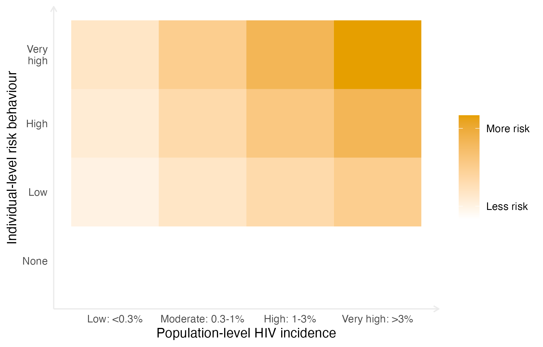
Figure 5.1: Risk of acquiring HIV depends on both individual-level risk behaviour and population-level HIV incidence. It is assumed here that with no individual-level risk behaviour, there is no risk of acquiring HIV, independent of the population-level HIV incidence. The risk scale is intended to be illustrative, rather than interpreted quantitatively.
In SSA, adolescent girls and young women (AGYW) aged 15-29 are at increased risk of HIV infection. AGYW account for only 28% of the population, but comprise 44% of new infections (UNAIDS 2021a). HIV incidence for AGYW is 2.4 times higher than for similarly aged (15-29) males. The social and biological reasons for this disparity include structural vulnerabilities and power imbalances, age patterns of sexual mixing, a younger age at first sex, and increased susceptibility to HIV infection. On this basis, AGYW have been identified as a priority population for HIV prevention services. Significant investments, including by the Global Fund (The Global Fund 2018) and the DREAMS (Determined, Resilient, Empowered, AIDS-free, Mentored, and Safe) partnership (Saul et al. 2018), have been made to support prevention programming.
The Global AIDS Strategy 2021-2026 (UNAIDS 2021b) was adopted by the United Nations (UN) General Assembly in June 2021, and “outlines the strategic priorities and actions to be implemented by global, regional, country and community partners to get on-track to ending AIDS”. It proposed stratifying HIV prevention packages to AGYW based on two factors:
- local population-level HIV incidence, and
- individual-level sexual risk behaviour.
Risk of acquiring HIV depends importantly on both factors. As such, prioritisation of prevention services is more efficient if both are taken into account. Figure 5.1 illustrates this fact stylistically. The strategy encourages programmes to define targets for the proportion of AGYW to be reached with a range of interventions (Table B.2) based on prioritisation strata which incorporate behavioural risk (Table B.1). Implementation of the strategy by national HIV programmes and stakeholders requires estimates of the population size and HIV incidence in each risk group by location.
In this chapter, I used a Bayesian spatio-temporal model (Section 5.3) of behavioural data from household surveys (Section 5.2) to estimate HIV risk group proportions. To then estimate risk group specific HIV prevalence and HIV incidences (Section 5.4), I combined the proportion estimates with population size, HIV prevalence and HIV incidence estimates, as well as risk group specific HIV incidence rate ratios, and HIV prevalence rate ratios. Finally, by ordering district, age, risk group strata by HIV incidence, I estimated an upper bound for the number of new HIV infections that could be averted under different risk prioritisation strategies (Section 5.4.3).
5.2 Data
5.2.1 Behavioural data from household surveys
I used household survey data from 13 countries identified by the Global Fund (The Global Fund 2018) as priority countries for implementation of AGYW HIV prevention. These countries were Botswana, Cameroon, Kenya, Lesotho, Malawi, Mozambique, Namibia, South Africa, Eswatini, Tanzania, Uganda, Zambia and Zimbabwe. Surveys conducted in these countries between 1999 and 2018 were included in which both women were interviewed about their sexual behaviour, and sufficient geographic data were available to locate survey clusters to health districts. There were 46 suitable surveys (Figure 5.2), with a total sample size of 274,970 women aged 15-29 years. Of the respondents, 103,063 were aged 15-19 years, 92,173 were aged 20-24 years, and 79,734 were aged 25-29 years. The median number of surveys per country was four, ranging from one in both Botswana and South Africa to six in Uganda.
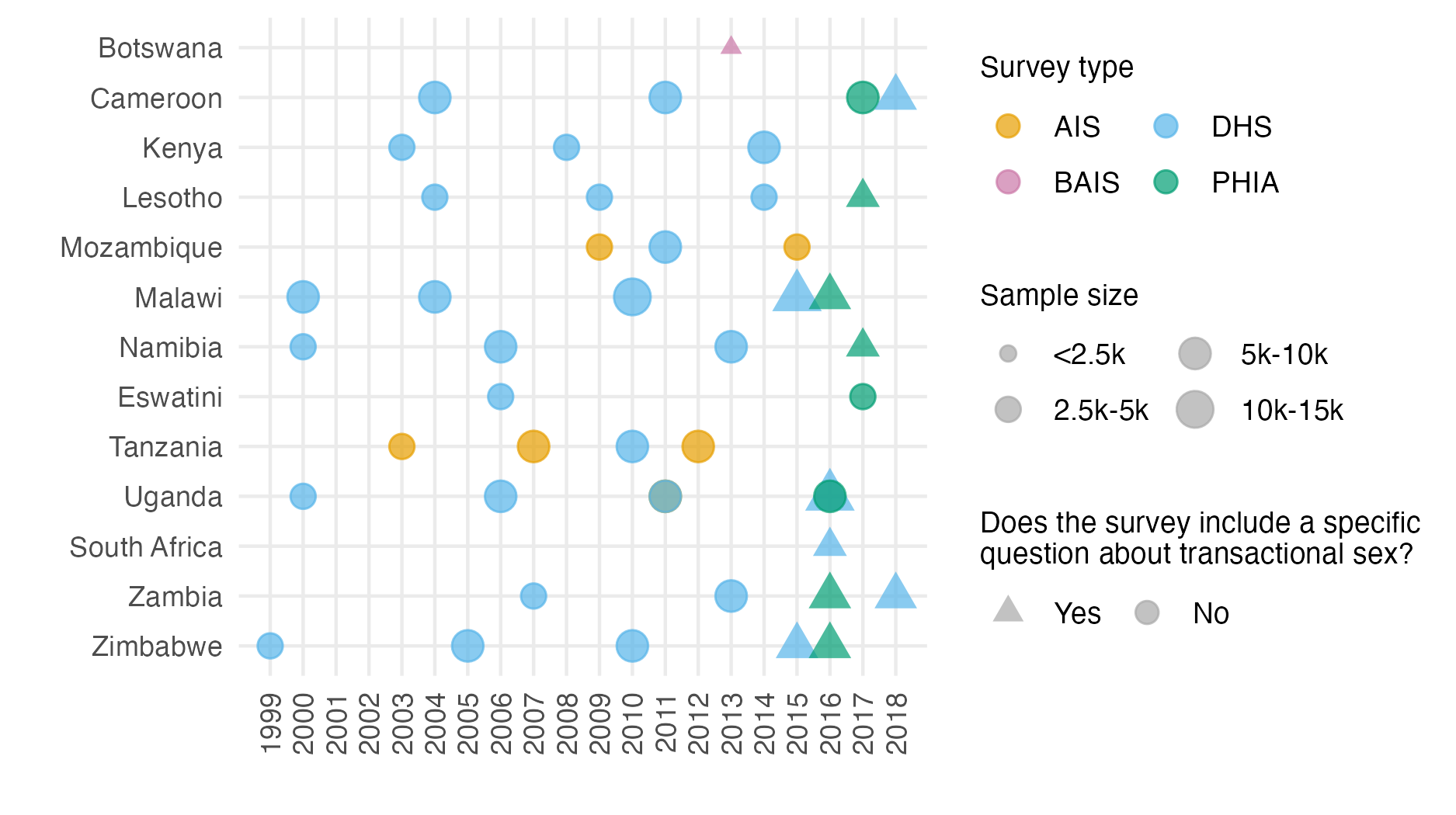
Figure 5.2: Surveys conducted 1999-2018 that were used in the analysis by year, survey type, sample size, and whether the survey included a specific question about transactional sex. That is, whether the respondent had “had sex in return for gifts, cash or anything else in the past 12 months”. Survey type included AIDS Indicator Surveys (AIS), Demographic and Health Surveys (DHS), the Botswana AIDS Impact Survey 2013 (BAIS), and Population-based HIV Impact Assessment (PHIA) surveys.
For each survey, respondents were classified into one of four behavioural risk groups according to reported sexual risk behaviour in the past 12 months (Figure 5.3), which I index by \(k\). In increasing order of HIV acquisition risk, these risk groups were:
- \(k = 1\): Not sexually active
- \(k = 2\): One cohabiting sexual partner
- \(k = 3\): Non-regular or multiple sexual partner(s), and
- \(k = 4\): Reporting transactional sex.
| Risk group | Description | Incidence rate ratio |
|---|---|---|
| None | Not sexually active | 0.0 |
| Low | One cohabiting sexual partner | 1.0 (baseline) |
| High | Non-regular or multiple partner(s) | 1.72 |
| Very High | Reporting transactional sex (later adjusted to correspond to FSW) | 3.0-25.0 (varied depending on local HIV incidence) |
The HIV incidence rate ratio \(\text{RR}_k\), used to calculate HIV incidence, was assumed to vary by risk group (Table 5.1). The one cohabiting partner risk group was set as baseline such that \(\text{RR}_2 = 1\). For the \(k = 4\) risk group, the HIV incidence ratio ratio was further assumed to vary by local HIV incidence among the general population.
Exact survey questions varied slightly across survey types and between survey phases. Questions captured information about whether the respondent had been sexually active in the past twelve months, and if so with how many partners. For their three most recent partners, respondents were also asked about the type of partnership. Possible partnership types included spouse, cohabiting partner, partner not cohabiting with respondent, friend, sex worker, sex work client, and other. The survey questions used are in Appendix B.4. In the case of inconsistent responses, women were categorised according to the highest risk group they fell into, ensuring that the categories were mutually exclusive.
Some surveys included a specific question asking if the respondent had received or given money or gifts for sex in the past twelve months. In these surveys, 2.64% of women reported transactional sex. In surveys without such a question, women almost never (0.01%) answered that one of their three most recent partners was a sex work client. This incomparability made it inappropriate to include surveys without a specific transactional sex question when estimating the proportion of the population who engaged in transactional sex. Of the total 46 surveys included in the analysis, 12 had a specific transactional sex question, with a total sample size of 62,853 (28,753 aged 15-19 years, 26,324 aged 20-24 years, and 7,776 aged 25-29 years). The sample size for women aged 25-29 is smaller because there were 6 DHS surveys which excluded women 25-29 from the transactional sex survey question. Table B.3 gives the sample size by age group for every survey included in the analysis.
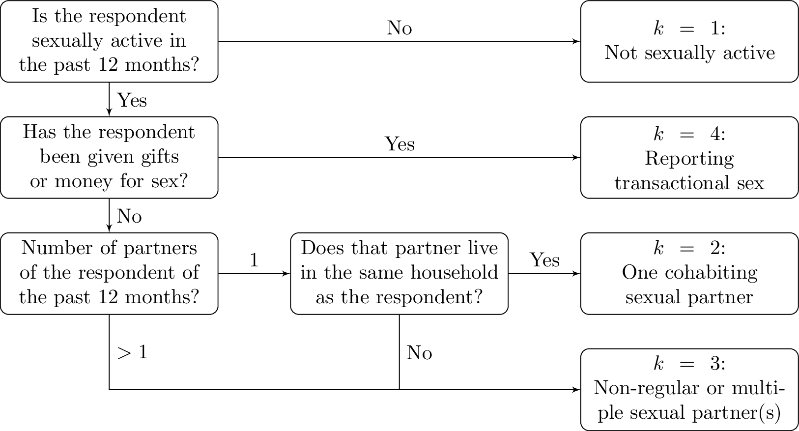
Figure 5.3: Flowchart describing how respondents were classified to HIV risk groups based on their survey responses.
5.2.2 Other data
In addition to the household survey behavioural data, I used estimates of population, PLHIV and new HIV infections stratified according to district and age group from HIV estimates published by UNAIDS that were developed using the Naomi model (Eaton et al. 2021). I used the most recent 2022 estimates for all countries, apart from Mozambique where, due to data accuracy concerns, I used the 2021 estimates (in which the Cabo Delgado province is excluded due to disruption by conflict). I used administrative area hierarchy and geographic boundaries corresponding to those used for health service planning by countries (Table B.5). Exceptions were Cameroon and Kenya, where I conducted analyses one level higher at the department and county levels, respectively.
5.3 Model for risk group proportions
Owing to the incomparability in estimating the \(k = 4\) risk group across surveys, I took a two-stage modelling approach to estimate the four risk group proportions. Denote being in either the third or fourth risk group as \(k = 3^{+}\). First, using all the surveys, I used a spatio-temporal multinomial logistic regression model to estimate the proportion of AGYW in the risk groups \(k \in \{1, 2, 3^{+}\}\). This model is described in Section 5.3.1. Then, using only those surveys with a specific transactional sex question, I fit a spatial logistic regression model to estimate the proportion of those in the \(k = 3^{+}\) risk group that were in the \(k = 3\) and \(k = 4\) risk groups respectively. This model is described in Section 5.3.2.
5.3.1 Spatio-temporal multinomial logistic regression
Let \(i \in \{1, \ldots, n\}\) denote districts partitioning the 13 studied AGYW priority countries \(c[i] \in \{1, \ldots, 13\}\). Consider the years 1999-2018 denoted as \(t \in \{1, \ldots, T\}\), and age groups \(a \in \{\text{15-19}, \text{20-24}, \text{25-29}\}\). Let \(p_{itak} > 0\) with \(\sum_{k = 1}^{3^{+}} p_{itak} = 1\), be the probabilities of membership of risk group \(k\).
5.3.1.1 Multinomial logistic regression
A standard multinomial logistic regression model (e.g. Gelman et al. 2013) is specified by \[\begin{align} \mathbf{y}_{ita} &= (y_{ita1}, \ldots, y_{ita3^{+}})^\top \sim \text{Multinomial}(m_{ita}; \, p_{ita1}, \ldots, p_{ita3^{+}}), \tag{5.1} \\ \log \left( \frac{p_{itak}}{p_{ita1}} \right) &= \eta_{itak}, \quad k = 2, 3^{+}, \tag{5.2} \end{align}\] where the number in risk group \(k\) is \(y_{itak}\), the fixed sample size is \(m_{ita} = \sum_{k = 1}^{3^{+}} y_{itak}\), and \(k = 1\) is chosen as the baseline category. This model is not a latent Gaussian model [LGM; Håvard Rue, Martino, and Chopin (2009)] because each observation \(y_{itak}\) for \(k \in \{1, 2, 3^{+}\}\) depends non-linearly on multiple structured additive predictors \(\{\eta_{itak}, k = 1, 2, 3^{+}\}\).
The model, defined over 940 districts, 20 years, 3 age groups, and 3 risk groups, is too large for MCMC to be tractable in reasonable time.
To recast this model as an LGM, I used the multinomial-Poisson transformation (detailed in Section 5.3.1.2).
This modification allowed inference to be performed using the INLA (Håvard Rue, Martino, and Chopin 2009) algorithm via the R-INLA package (Martins et al. 2013).
5.3.1.2 The multinomial-Poisson transformation
The multinomial-Poisson transformation (Baker 1994) reframes a given multinomial logistic regression model, like that described in Equations (5.1) and (5.2), as an equivalent Poisson log-linear model. The equivalent model is of the form \[\begin{align} y_{itak} &\sim \text{Poisson}(\kappa_{itak}), \tag{5.3} \\ \log(\kappa_{itak}) &= \eta_{itak}. \tag{5.4} \end{align}\] The basis of the transformation is that conditional on their sum Poisson counts are jointly multinomially distributed (McCullagh and Nelder 1989) as follows \[\begin{equation} \mathbf{y}_{ita} \, | \, m_{ita} \sim \text{Multinomial} \left( m_{ita}; \frac{\kappa_{ita1}}{\kappa_{ita}}, \ldots, \frac{\kappa_{ita3^{+}}}{\kappa_{ita}} \right), \tag{5.5} \end{equation}\] where \(\kappa_{ita} = \sum_{k = 1}^{3^{+}} \kappa_{itak}\). The probabilities \(p_{itak}\) may then be obtained using the softmax function \[\begin{equation} p_{itak} = \frac{\exp(\eta_{itak})}{\sum_{k = 1}^{3^{+}} \exp(\eta_{itak})} = \frac{\kappa_{itak}}{\sum_{k = 1}^{3^{+}} \kappa_{itak}} = \frac{\kappa_{itak}}{\kappa_{ita}}. \end{equation}\] Under the equivalent model, in Equation (5.3) the sample sizes \(m_{ita}\) are treated as random rather than fixed such that \[\begin{equation} m_{ita} = \sum_k y_{itak} \sim \text{Poisson} \left( \sum_k \kappa_{itak} \right) = \text{Poisson} \left( \kappa_{ita} \right). \tag{5.6} \end{equation}\] Using Equations (5.5) for \(p(\mathbf{y}_{ita} \, | \, m_{ita})\) and Equation (5.6) for \(p(m_{ita})\), the joint distribution is given by \[\begin{align} p(\mathbf{y}_{ita}, m_{ita}) &= \exp(-\kappa_{ita}) \frac{(\kappa_{ita})^{m_{ita}}}{m_{ita}!} \times \frac{m_{ita}!}{\prod_k y_{itak}!} \prod_k \left( \frac{\kappa_{itak}}{\kappa_{ita}} \right)^{y_{itak}} \\ &= \prod_k \left( \frac{\exp(-\kappa_{itak}) \left( \kappa_{itak} \right)^{y_{itak}}}{y_{itak}!} \right) \\ &= \prod_k \text{Poisson} \left( y_{itak} \, | \, \kappa_{itak} \right). \tag{5.7} \end{align}\] As expected, Equation (5.7) corresponds to the product of independent Poisson likelihoods defined in Equation (5.3). This exercise demonstrates that the Poisson log-linear model contains within it a multinomial likelihood, with a Poisson prior on the sample size.
For this model to be equivalent to a multinomial logistic regression model, the normalisation constants \(m_{ita}\) must be recovered exactly. That is to say, their posterior distributions should be as close as possible to a Dirac delta distribution with value zero everywhere but the known value of the sample size. To ensure that this is the case, observation-specific random effects \(\theta_{ita}\) can be included in the equation for the linear predictor. Multiplying each of \(\{\kappa_{itak}\}_{k = 1}^{3^+}\) by \(\exp(\theta_{ita})\) has no effect on the category probabilities, but does provide the necessary flexibility for \(\kappa_{ita}\) to recover \(m_{ita}\) exactly. Although in theory an improper prior distribution \(\theta_{ita} \propto 1\) should be used, I found that in practice, by keeping \(\eta_{ita}\) otherwise small using appropriate constraints, so that arbitrarily large values of \(\theta_{ita}\) are not required, it is sufficient (and practically preferable for inference) to instead use a vague prior distribution.
5.3.1.3 Model specifications
I considered four models (Table 5.2) for \(\eta_{ita}\) in the equivalent Poisson log-linear model of the form \[\begin{equation} \eta_{ita} = \theta_{ita} + \beta_k + \zeta_{c[i]k} + \alpha_{ac[i]k} + u_{ik} + \gamma_{tk}. \end{equation}\] Observation random effects \(\theta_{ita} \sim \mathcal{N}(0, 1000^2)\) with a vague prior distribution were included in all models to ensure the multinomial-Poisson transformation was valid. To capture country-specific proportion estimates for each category, I included category random effects \(\beta_k \sim \mathcal{N}(0, \tau_\beta^{-1})\) and country-category random effects \(\zeta_{ck} \sim \mathcal{N}(0, \tau_\zeta^{-1})\). Heterogeneity in risk group proportions by age was allowed by including age-country-category random effects \(\alpha_{ack} \sim \mathcal{N}(0, \tau_\alpha^{-1})\). Several specifications were considered for the space-category \(u_{ik}\) and time-category effects \(\gamma_{tk}\), described in Sections 5.3.1.3.1 and 5.3.1.3.2.
| Category \(\beta_k\) | Country \(\zeta_{ck}\) | Age \(\alpha_{ack}\) | Spatial \(u_{ik}\) | Temporal \(\gamma_{tk}\) | |
|---|---|---|---|---|---|
| M1 | IID | IID | IID | IID | IID |
| M2 | IID | IID | IID | Besag | IID |
| M3 | IID | IID | IID | IID | AR1 |
| M4 | IID | IID | IID | Besag | AR1 |
Use of the multinomial-Poisson transformation required all random effects to include interaction with category \(k\), because any random effects which did not include interaction with category would give no change in category probabilities. The only exception were the observation random effects, which were included as a device to ensure the transformation is valid, rather than to model the data.
5.3.1.3.1 Spatial random effects
For the space-category random effects \(u_{ik}\) I considered two specifications:
- Independent and identically distributed (IID) \(u_{ik} \sim \mathcal{N}(0, \tau_u^{-1})\),
- The Besag improper conditional autoregressive (ICAR) model (Besag, York, and Mollié 1991) grouped by category
\[
\mathbf{u} = (u_{11}, \ldots, u_{n1}, \ldots, u_{1{3^{+}}}, \ldots u_{n3^{+}})^\top \sim \mathcal{N}(\mathbf{0}, (\tau_u \mathbf{R}^\star_u)^{-}).
\]
The scaled structure matrix \(\mathbf{R}^\star_u = \mathbf{R}^\star_b \otimes \mathbf{I}\) is given by the Kronecker product of the scaled Besag structure matrix \(\mathbf{R}^\star_b\) and the identity matrix \(\mathbf{I}\), and \(\mathbf{A}^{-}\) denotes the generalised matrix inverse of \(\mathbf{A}\)
I followed best practices for the Besag model as described in Chapter 4.
To implement the Kronecker product I used the
groupoption inR-INLA[Section 3.5.5; Gómez-Rubio (2020)] setting the random effect to bef(area_idx, model = "besag", group = cat_idx, control.group = list(model = "iid"), ...). Though the Kronecker product is symmetric, performance is better inR-INLAwhen the more complicated effect is written as the first variable rather than the grouping variable.
In preliminary testing I used the BYM2 model (Simpson et al. 2017) in place of the Besag. I found that the proportion parameter posteriors tended to be highly peaked at the value one. For simplicity and to avoid numerical issues, by using Besag random effects I effectively decided to fix this proportion to one.
5.3.1.3.2 Temporal random effects
For the time-category random effects \(\gamma_{tk}\) I considered two specifications:
- IID \(\gamma_{tk} \sim \mathcal{N}(0, \tau_\gamma^{-1})\),
- First order autoregressive (AR1) grouped by category
\[
\boldsymbol{\mathbf{\gamma}} = (\gamma_{11}, \ldots, \gamma_{13^{+}}, \ldots, \gamma_{T1}, \ldots, \gamma_{T3^{+}})^\top \sim \mathcal{N}(\mathbf{0}, (\tau_\gamma \mathbf{R}^\star_\gamma)^{-}).
\]
The scaled structure matrix \(\mathbf{R}^\star_\gamma = \mathbf{R}^\star_r \otimes \mathbf{I}\) is given by the Kronecker product of a scaled AR1 structure matrix \(\mathbf{R}^\star_r\) and the identity matrix \(\mathbf{I}\).
The AR1 structure matrix \(\mathbf{R}_r\) is obtained by the precision matrix of the random effects \(\mathbf{r} = (r_1, \ldots, r_T)^\top\) specified by
\[\begin{align}
r_1 &\sim \left( 0, \frac{1}{1 - \rho^2} \right), \\
r_t &= \rho r_{t - 1} + \epsilon_t, \quad t = 2, \ldots, T,
\end{align}\]
where \(\epsilon_t \sim \mathcal{N}(0, 1)\) and \(|\rho| < 1\).
As with the structured spatial random effects, I implemented this Kronecker product using the
groupoption viaf(year_idx, model = "ar1", group = cat_idx, control.group = list(model = "iid"), ...). Again, the variable with the more complicated model was written first.
5.3.1.3.3 Note on spatio-temporal interaction random effects
I also considered including separable space-time-category random effects \(\delta_{itk}\) in the model, using the specification \[\begin{equation} \boldsymbol{\mathbf{\delta}} = (\delta_{111}, \ldots, \delta_{nT3^{+}})^\top \sim \mathcal{N}(\mathbf{0}, (\tau_\delta \mathbf{R}^\star_\delta)^{-}), \end{equation}\] where \(\mathbf{R}^\star_\delta\) is a Kronecker product of the relevant space, time and category structure matrices. These specifications were:
- IID spatial and IID temporal (Type I) \(\mathbf{R}^\star_\delta = \mathbf{I} \otimes \mathbf{I} \otimes \mathbf{I}\),
- Besag spatial and IID temporal (Type II) \(\mathbf{R}^\star_\delta = \mathbf{R}^\star_b \otimes \mathbf{I} \otimes \mathbf{I}\),
- IID spatial and AR1 temporal (Type III) \(\mathbf{R}^\star_\delta = \mathbf{I} \otimes \mathbf{R}^\star_a \otimes \mathbf{I}\),
- Besag spatial and AR1 (Type IV) \(\mathbf{R}^\star_\delta = \mathbf{R}^\star_b \otimes \mathbf{R}^\star_a \otimes \mathbf{I}\),
where the first, second and third elements of the Kronecker product represent space, time and category (always IID) structure matrices respectively. The interaction type in brackets (e.g. Type I) is given according to the Knorr-Held (2000) framework.
Though three-way Kronecker products are not directly supported in R-INLA, I implemented each specification using a combination of the group and replicate options [Section 6.5.2; Gómez-Rubio (2020)].
For example, for the Type IV effects the random effects were specified by f(area_idx_copy, model = "besag", group = year_idx, replicate = cat_idx, control.group = list(model = "ar1")).
I was able to run these models for single countries, keeping only years at which surveys occurred in those countries.
However, when fitting all countries jointly I found inclusion of the space-time-category random effects to be intractable, and as such decided not to include them in the model.
5.3.1.3.4 Prior distributions
All random effect precision parameters \[\begin{equation} \tau \in \{\tau_\beta, \tau_\zeta, \tau_\alpha, \tau_u, \tau_\gamma, \tau_\delta\} \end{equation}\] were given independent penalised complexity (PC) prior distributions (Simpson et al. 2017) with base model \(\sigma = 0\) given by \[\begin{equation} p(\tau) = 0.5 \nu \tau^{-3/2} \exp \left( - \nu \tau^{-1/2} \right), \end{equation}\] where \(\nu = - \ln(0.01) / 2.5\) such that \(\mathbb{P}(\sigma > 2.5) = 0.01\). For the lag-one correlation parameter \(\rho\), I used the PC prior distribution, as derived by Sørbye and Rue (2017), with base model \(\rho = 1\) and condition \(\mathbb{P}(\rho > 0 = 0.75)\). I chose the base model \(\rho = 1\) corresponding to no change in behaviour over time, rather than the alternative \(\rho = 0\) corresponding to no correlation in behaviour over time, as I judged the former to be more plausible a priori.
5.3.1.4 Identifiability constraints
To facilitate interpretability of the posterior inferences, I applied sum-to-zero constraints (Table 5.3) such that none of the category interaction random effects altered overall category probabilities.
In testing of the space-time-category random effects, I applied analogous sum-to-zero constraints to maintain roles of the space-category and time-category random effects.
In some cases it was not possible to implement all three sets of constraints for the three-way interactions in R-INLA.
| Random effects | Constraints |
|---|---|
| Category | \(\sum_k \beta_k = 0\) |
| Country | \(\sum_c \zeta_{ck} = 0, \, \forall \, k\) |
| Age-country | \(\sum_a \alpha_{ack} = 0, \, \forall \, c, k\) |
| Spatial | \(\sum_i u_{ik} = 0, \, \forall \, k\) |
| Temporal | \(\sum_t \gamma_{tk} = 0, \, \forall \, k\) |
| Spatio-temporal | \(\sum_i \delta_{itk} = 0, \, \forall \, t, k; \sum_t \delta_{itk} = 0, \, \forall \, i, k; \sum_k \delta_{itk} = 0, \, \forall \, i, t\) |
5.3.1.5 Survey weighted likelihood
I accounted for the survey design using a weighted pseudo-likelihood where the observed counts \(y\) are replaced by effective counts \(y^\star\), as described in Section 3.5.
These counts may not be integers, and as such the Poisson likelihood given in Equation (5.3) is not appropriate.
Instead, I used a generalised Poisson pseudo-likelihood \(y^\star \sim \text{xPoisson}(\kappa)\) given by
\[\begin{equation}
p(y^\star) = \frac{\kappa^{y^\star}}{\left \lfloor{y^\star!}\right \rfloor } \exp \left(- \kappa \right),
\end{equation}\]
to extend the Poisson distribution to non-integer weighted counts.
This working likelihood is implemented by family = "xPoisson" in R-INLA.
5.3.1.6 Model selection
I selected the model including Besag spatial random effects and IID temporal random effects based on the conditional predictive ordinate (CPO) criterion (Pettit 1990).
For comparison, I also computed the deviance information criterion (DIC) (D. J. Spiegelhalter et al. 2002) and widely applicable information criterion (WAIC) (Watanabe 2013).
Each of these criterion can be calculated in R-INLA without requiring model refitting.
The results are presented in Table 5.4 and Figure 5.4.
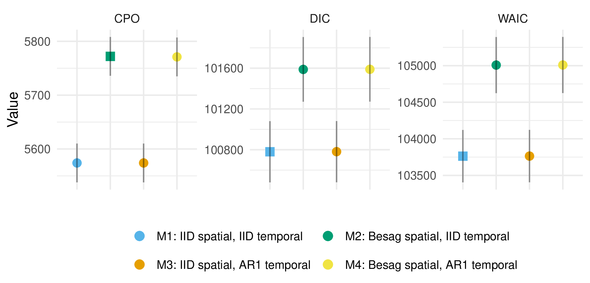
Figure 5.4: For the multinomial logistic regression model, under the conditional predictive ordinate (CPO) criterion, including Besag spatial random effects rather than IID spatial random effects improved model performance. On the other hand, under the deviance information criterion (DIC) and widely applicable information criterion (WAIC), where smaller values are preferred, the opposite was true. The relatively poor DIC and WAIC performance of Besag random effects was due to outlying values of these criteria for three of four surveys in Tanzania, and as such may be erroneous. Though IID temporal random effects are preferred by all criteria, AR1 temporal random effects performed very similarly, likely as there is a limited amount of temporal variation in the data to describe.
| M1 | M2 | M3 | M4 | |
|---|---|---|---|---|
| CPO | 5573 (36) | 5772 (36) | 5574 (36) | 5771 (36) |
| DIC | 100780 (300) | 101588 (317) | 100781 (300) | 101589 (317) |
| WAIC | 103763 (358) | 105008 (383) | 103763 (358) | 105009 (383) |
5.3.2 Spatial logistic regression
To estimate the proportion of those in the \(k = 3^{+}\) risk group that were in the \(k = 3\) and \(k = 4\) risk groups respectively, I fit logistic regression models of the form \[\begin{align} y_{ia4} &\sim \text{Binomial} \left( y_{ia3} + y_{ia4}, q_{ia} \right), \tag{5.8} \\ q_{ia} &= \text{logit}^{-1} \left( \eta_{ia} \right), \end{align}\] where \[\begin{equation} q_{ia} = \frac{p_{ia4}}{p_{ia3} + p_{ia4}} = \frac{p_{ia4}}{p_{ia{3^+}}}. \end{equation}\] This two-step approach allowed all surveys to be included in the multinomial regression model, but only those surveys with a specific transactional sex question to be included in the logistic regression model. As all such surveys occurred in the years 2013-2018 (Figure 5.2) I assumed no dependence on time, hence omission of the index \(t\). Model specification for the linear predictor \(\eta_{ia}\) is discussed in Section 5.3.2.1 to follow.
5.3.2.1 Model specifications
| Intercept \(\beta_0\) | Country \(\zeta_{c}\) | Age \(\alpha_{ac}\) | Spatial \(u_{i}\) | Covariates | |
|---|---|---|---|---|---|
| L1 | Constant | IID | IID | IID | None |
| L2 | Constant | IID | IID | Besag | None |
| L3 | Constant | IID | IID | IID | cfswever |
| L4 | Constant | IID | IID | Besag | cfswever |
| L5 | Constant | IID | IID | IID | cfswrecent |
| L6 | Constant | IID | IID | Besag | cfswrecent |
I considered six logistic regression models (Table 5.5). Each included a constant intercept \(\beta_0 \sim \mathcal{N}(-2, 1^2)\), country random effects \(\zeta_{c} \sim \mathcal{N}(0, \tau_\zeta^{-1})\), and age-country random effects \(\alpha_{ac} \sim \mathcal{N}(0, \tau_\alpha^{-1})\). The Gaussian prior distribution on \(\beta_0\) placed 95% prior probability on the range 2-50% for the percentage of those with non-regular or multiple partners who report transactional sex. I considered two specifications (IID, Besag) for the spatial random effects \(u_i\). To aid estimation with sparse data, I also considered national-level covariates for the proportion of men who have paid for sex ever or in the last twelve months (Hodgins et al. 2022). For both random effect precision parameters \(\tau \in \{\tau_\alpha, \tau_\zeta\}\) I used the PC prior distribution with base model \(\sigma = 0\) and \(\mathbb{P}(\sigma > 2.5 = 0.01)\). For both regression parameters \(\beta \in \{\beta_\texttt{cfswever}, \beta_\texttt{cfswrecent}\}\) I used the prior distribution \(\beta \sim \mathcal{N}(0, 2.5^2)\).
5.3.2.2 Survey weighted likelihood
As with the multinomial regression model, I used survey weighted counts \(y^\star\) and sample sizes \(m^\star\).
I used a generalised binomial pseudo-likelihood \(y^\star \sim \text{xBinomial}(m^\star, q)\) given by
\[\begin{equation}
p(y^\star \, | \, m^\star, q) = \binom{\lfloor m^\star \rfloor}{\lfloor y^\star \rfloor} q^{y^\star} (1 - q)^{m^\star - y^\star}
\end{equation}\]
to extend the binomial distribution to non-integer weighted counts and sample sizes.
This working likelihood is implemented by family = "xBinomial" in R-INLA.
5.3.2.3 Model selection
I selected the model including Besag spatial effects and cfswrecent covariates according to the CPO criterion.
All results, including DIC and WAIC, are presented in Table 5.6 and Figure 5.5.
Inclusion of Besag spatial random effects, rather than IID, consistently improved performance.
Benefits from inclusion of covariates were more marginal.
As some countries had no suitable surveys, I nonetheless preferred to include covariate information so that estimates in these countries would be based on some country-specific data.
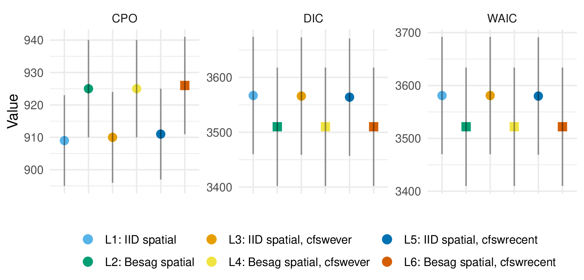
Figure 5.5: For the logistic regression model, the CPO, DIC, and WAIC each agreed that the model containing Besag spatial random effects and the cfswrecent covariates was best. Inclusion of Besag spatial random effects consistently improved each criterion, whereas improvements from inclusion of any covariates were marginal.
| L1 | L2 | L3 | L4 | L5 | L6 | |
|---|---|---|---|---|---|---|
| CPO | 950 (15) | 969 (15) | 951 (15) | 970 (15) | 950 (15) | 970 (15) |
| DIC | 4662 (110) | 4605 (111) | 4662 (110) | 4605 (111) | 4662 (110) | 4605 (111) |
| WAIC | 4692 (115) | 4624 (115) | 4692 (115) | 4624 (115) | 4692 (115) | 4624 (115) |
5.3.3 Female sex worker population size adjustment
Domain experts do not consider having had sex “in return for gifts, cash or anything else in the past 12 months” sufficient to constitute sex work. For this reason, I adjusted the estimates obtained based on the transactional sex survey question to match alternatively obtained age-country FSW population size estimates. Taking this approach retained subnational variation informed by the transactional sex survey question.
I used the estimates of adult (15-49) FSW population size by country from a Bayesian meta-analysis of key population specific data sources (Stevens et al. 2023). To disaggregate these estimates by age, I took the following steps. First, I calculated the total sexually debuted population in each age group, by country. To describe the distribution of age at first sex, I used skew logistic distributions (Nguyen and Eaton 2022) with cumulative distribution function given by \[\begin{equation} F(x) = \left(1 + \exp(\kappa_c (\mu_c - x)) \right)^{- \gamma_c}, \end{equation}\] where \(\kappa_c, \mu_c, \gamma_c > 0\) are country-specific shape, shape and skewness parameters respectively. Next, I used the assumed \(\text{Gamma}(\alpha = 10.4, \beta = 0.36)\) FSW age distribution in South Africa from the Thembisa model (L. Johnson and Dorrington 2020) to calculate the implied ratio between the number of FSW and the sexually debuted population in each age group. I assumed the South African ratios were applicable to every country, allowing calculation of the number of FSW by age group in all 13 countries. The resulting age trends obtained (Figure 5.6) reflect country-level variation in demographics and age-at-first-sex.
Altering the FSW population size estimates requires that other risk group population size estimates are also altered such that the corresponding risk group proportion estimates sum to one. Here, estimates of the non-regular or multiple sexual partner(s) population size were altered to facilitate changing of the FSW population size.
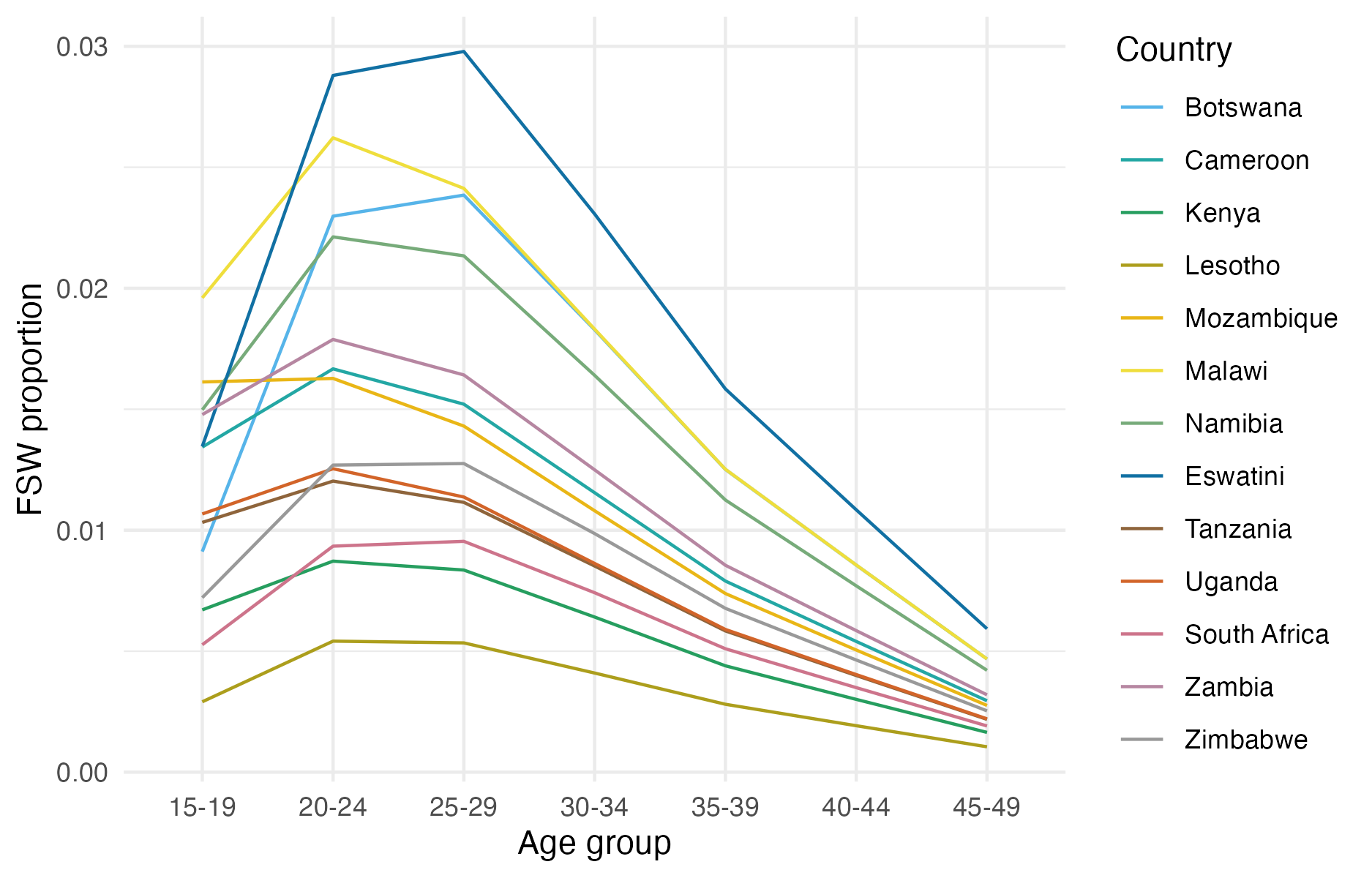
Figure 5.6: The disaggregation procedure I used produces an age distribution for FSW peaking in the 20-24 and 25-29 age groups, and declining for older age groups.
5.4 Prevalence and incidence by risk group
Using the most recent risk group proportion estimates, I calculated the following indicators, stratified by district, age group and risk group:
- HIV prevalence \(\rho_{iak}\),
- the number of people living with HIV (PLHIV) \(H_{iak}\),
- HIV incidence \(\lambda_{iak}\), and
- the number of new HIV infections \(I_{iak}\).
To do so, I disaggregated district, age group specific Naomi estimates by risk group.
5.4.1 Disaggregation of Naomi prevalence estimates
To disaggregate HIV prevalence, I began by estimating HIV prevalence log odds ratios \(\log(\text{OR}_k)\) relative to the general population. To do so, I began by calculating age, country, and risk group specific (as well as general population) HIV prevalence \(\rho_{cak}\) using bio-marker survey data from all 46 surveys included in the risk group model (Section 5.2.1). I then fit a logistic regression model, with indicator functions for each risk group, and an indicator for being in the general population. The fitted regression coefficients in this model \(\beta_k\) correspond to log odds \(\log \rho_k - \log(1 - \rho_k)\). The required log odds ratios may then be easily obtained by taking the difference in odds ratios.
To allow the log odds ratio for the highest risk group to vary based on general population prevalence I fit a linear regression of the FSW log odds against the general population log odds. I ensured that log odds ratios for the FSW risk group were at least as large as those for the multiple or non-regular partner(s) risk group.
Given the fitted log odds ratios, I disaggregated Naomi estimates of PLHIV \(H_{ia}\) on the logit scale using numerical optimisation. To do so, I found the values of \(\theta_{ia}\) which minimised the equation \[\begin{equation} f(\theta_{ia}) = \sum_{k = 1}^4 \left( \text{logistic}(\theta_{ia} + \log(\text{OR}_k)) \cdot N_{iak} \right) - H_{ia}, \end{equation}\] where \(\text{logistic}(x) = \exp(x) / (1 + \exp(x))\) such that \(\text{logistic}(\hat \theta_{ia} + \log(\text{OR}_k)) = \rho_{iak}\). These values were given by \[\begin{equation} \hat \theta_{ia} = \arg\min_{\theta_{ia} \in [-10, 10]} f(\theta_{ia})^2. \end{equation}\] The number of PLHIV were obtained by \(H_{iak} = \rho_{iak} N_{iak}\), where \(N_{iak}\) is the risk group population size.
5.4.2 Disaggregation of Naomi incidence estimates
I used linear disaggregation to calculate the number of new HIV infections by risk group \[\begin{align} I_{ia} &= \sum_k I_{iak} = \sum_k \lambda_{iak} (1 - \rho_{iak}) N_{iak} \\ &= 0 + \lambda_{ia2} (1 - \rho_{ia2}) N_{ia2} + \lambda_{ia3} (1 - \rho_{ia3}) {ia3} + \lambda_{ia4} (1 - \rho_{ia4}) N_{ia4} \\ &= \lambda_{ia2} \left((1 - \rho_{ia2}) N_{ia2} + \text{RR}_{3} (1 - \rho_{ia3}) N_{ia3} + \text{RR}_4(\lambda_{ia}) (1 - \rho_{i4}) N_{ia4} \right), \end{align}\] where \(\text{RR}_{2}\), \(\text{RR}_{3}\) and \(\text{RR}_{4}(\cdot)\) are the HIV risk ratios given in Table 5.1, and \((1 - \rho_{iak}) N_{iak}\) are the susceptible population sizes in each risk group. The risk ratio for FSW was defined as a function of district-level incidence in the general population \(\lambda_{ia}\). Risk group specific HIV incidence estimates were then given by \[\begin{align} \lambda_{ia1} &= 0, \\ \lambda_{ia2} &= \frac{I_{ia}}{(1 - \rho_{ia2}) N_{ia2} + \text{RR}_{3} (1 - \rho_{ia3}) N_{ia3} + \text{RR}_4(\lambda_{ia}) (1 - \rho_{ia4}) N_{ia4}}, \\ \lambda_{ia3} &= \text{RR}_{3} \lambda_{ia2}, \\ \lambda_{ia4} &= \text{RR}_4(\lambda_{ia}) \lambda_{ia2}. \end{align}\] These equations were evaluated using Naomi model estimates of the number of new HIV infections \(I_{ia} = \lambda_{ia} N_{ia}\). The number of new HIV infections were \(I_{iak} = \lambda_{iak} N_{iak}\).
5.4.3 Expected new infections reached
To quantify the number of new infections that could be reached prioritising according to each possible stratification of the population, I took the following approach, which I illustrate for stratification by age. First, I aggregated the number of new HIV infections and HIV incidence (calculated above in Section 5.4.2) such that \[\begin{align} I_a &= \sum_{ik} I_{iak}, \\ \lambda_a &= I_a / \sum_{ik} (1 - \rho_{iak}) N_{iak}. \end{align}\] I then considered prioritisation individuals by age group \(a\) according to the highest HIV incidence \(\lambda_a\). By cumulatively summing the expected infections, for each fraction of the total population reached (0-100%) I calculated the fraction of total expected new infections that would be reached. In this instance, as there are three age groups, the resulting function was piecewise linear with three segments. This analysis was repeated for all \(2^3 = 8\) possible combinations of stratification by location, age, and risk group.
5.5 Results
5.5.1 Model for risk group proportions
5.5.1.1 Estimates
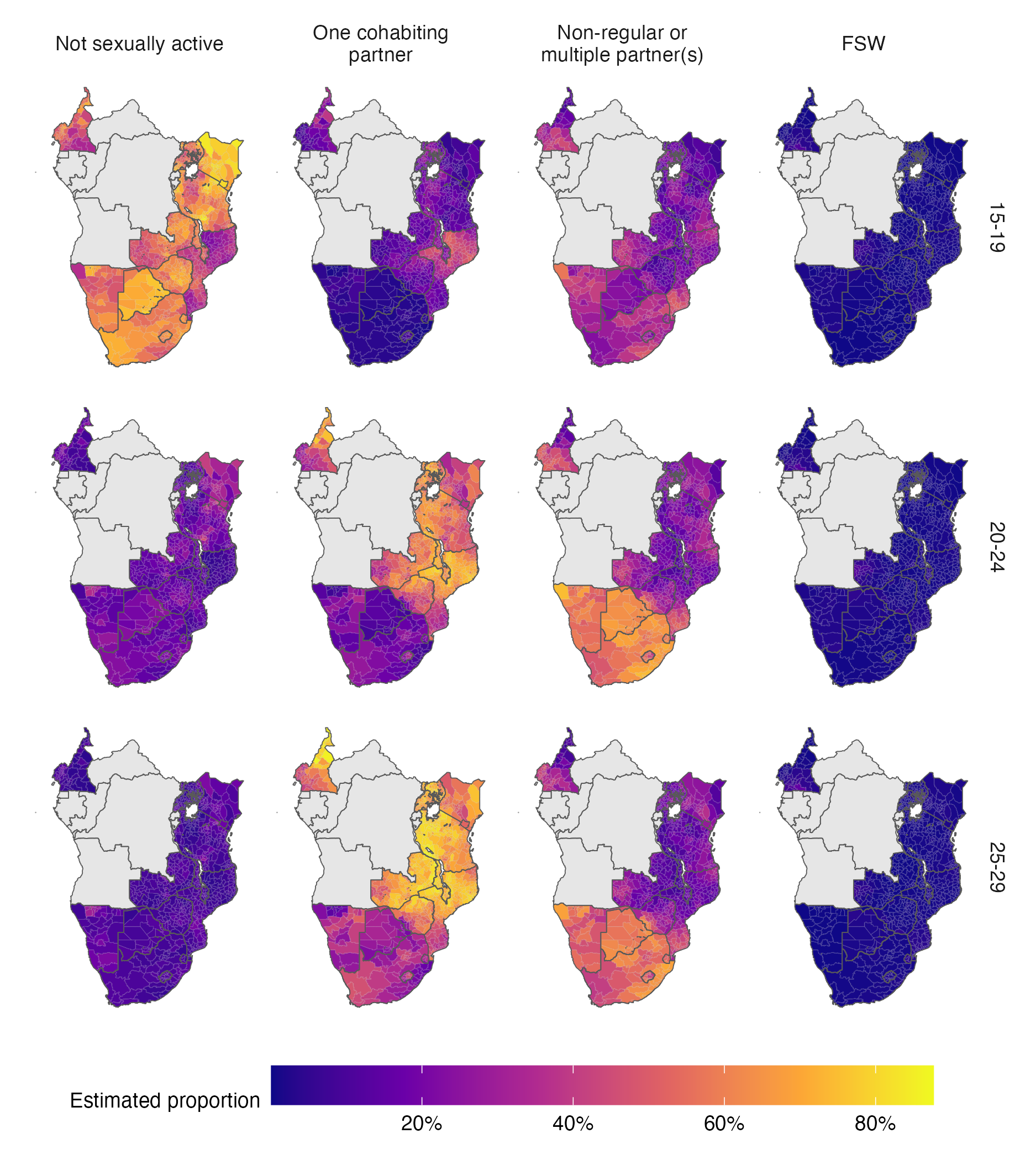
Figure 5.7: The posterior mean of the AGYW risk group proportions over space in 2018. Estimates are stratified by risk group (columns) and five-year age group (rows). Countries in grey were not included in the analysis. A limitation of this figure is that using a common colour scale, though desirable for other reasons, makes it challenging to see spatial variation in the FSW risk group.
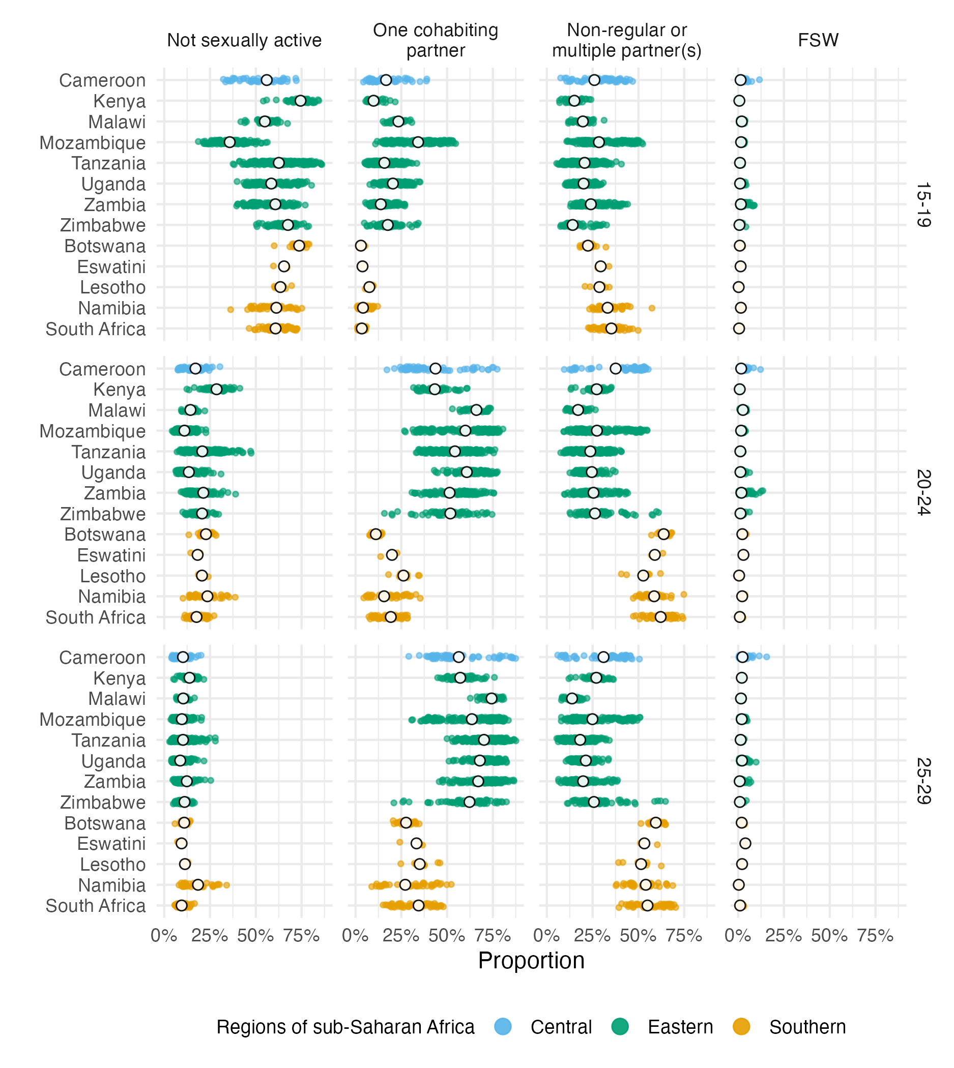
Figure 5.8: National (in white) and subnational (in color) posterior means of the risk group proportions. Estimates are stratified by risk group (columns) and five-year age group (rows). Though the information presented is similar to that of Figure 5.7, this figure presents a clear view of within- and between-country variation in risk group proportions.
Figure B.1 and Figure 5.8 show posterior mean estimates for the proportion in each risk group for the final model in 2018, the most recent year included in our analysis. I focused on the most recent estimates because they are the most relevant to inform ongoing HIV policy. In subsequent results, all estimates refer to 2018, unless otherwise indicated.
The median national FSW proportion was 1.1% (95% CI 0.4–1.9) for the 15-19 age group, 1.6% (95% CI 0.6–2.8) for the 20-24 age group and 1.9% (95% CI 0.5–3.5) for the 25-29 age group, in line with the results displayed in Figure 5.6.
In the 20-24 and 25-29 year age groups, the majority of women were either cohabiting or had non-regular or multiple partner(s). Countries in eastern and central Africa (Cameroon, Kenya, Malawi, Mozambique, Tanzania, Uganda, Zambia and Zimbabwe) had a higher proportion of women in these age groups cohabiting (63.1% [95% CI 35–78.7%] compared with 21.3% [95% CI 10.1–48.8%] with non-regular partner[s]). In contrast, countries in southern Africa (Botswana, Eswatini, Lesotho, Namibia and South Africa) had a higher proportion with non-regular or multiple partner(s) (58.9% [95% CI 43.2–70.5%], compared with 23.4% [95% CI 9.7–39.1%] cohabiting). This finding is the most notable feature of between-country variation shown in Figure 5.8. Figure 5.7 shows the geographic delineation to pass along the border of Mozambique, through the interior of Zimbabwe and along the border of Zambia. The bimodality of the 20-24 and 25-29 year age groups is shown in Figure B.2.
In the median district, 57.9% of adolescent girls 15-19 were not sexually active (95% credible interval [CI] at the district-level 27.7–79.7). The country of Mozambique was an exception, where the majority of adolescent girls 15-19 (64.23%) were sexually active in the past year and close to a third (34.17%) were cohabiting with a partner.
5.5.1.2 Coverage assessment
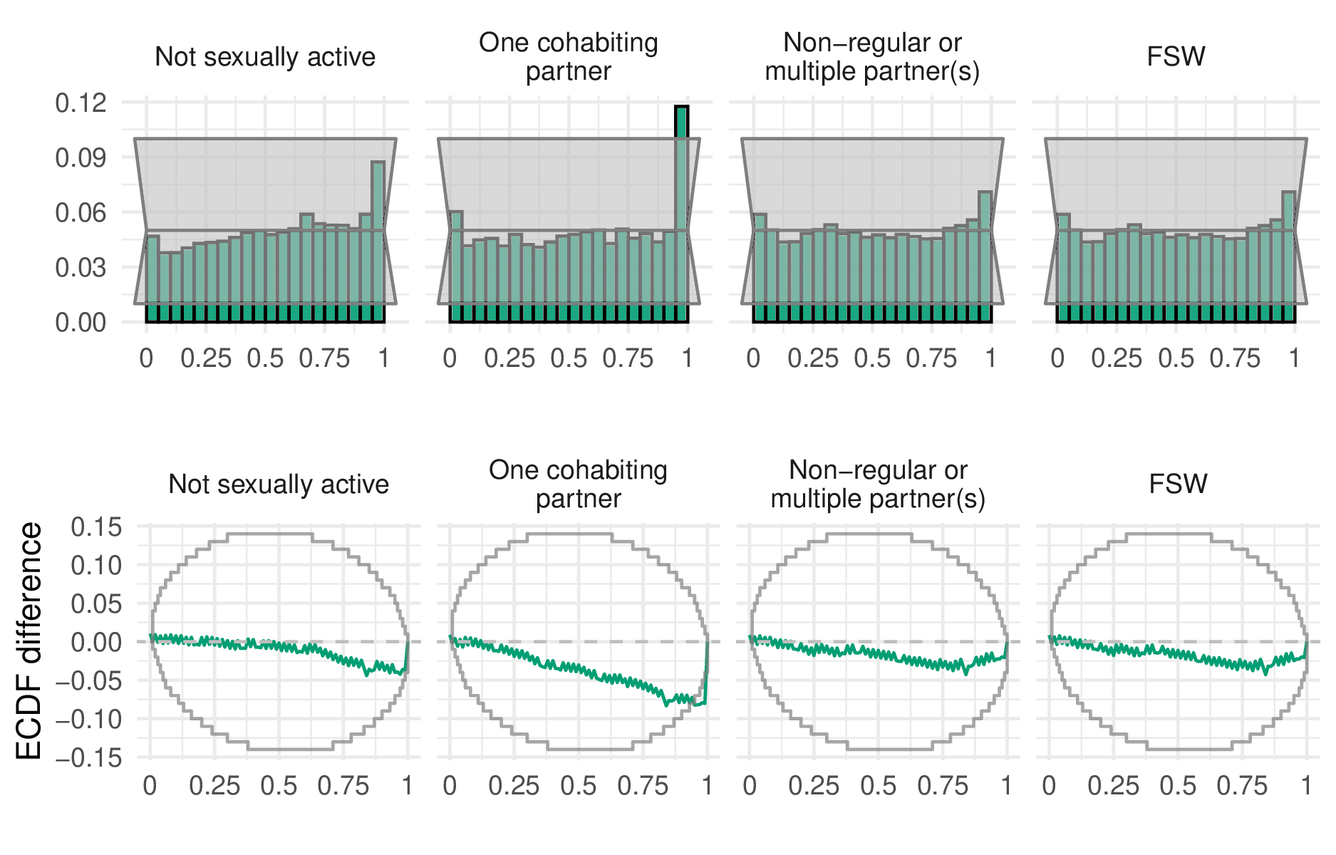
Figure 5.9: Probability integral transform (PIT) histograms (top row) and empirical cumulative distribution function (ECDF) difference plots (bottom row) for the final selected model.
To assess the calibration of the fitted model, I calculated the quantile \(q\) of each observation within the posterior predictive distribution. For calibrated models, these quantiles, known as probability integral transform (PIT) values (Dawid 1984; Nikos I. Bosse et al. 2022), should follow a uniform distribution \(q \sim \mathcal{U}[0, 1]\). To generate samples from the posterior predictive distribution, I applied the multinomial likelihood to samples from the latent field, setting the sample size to be the floor of the Kish effective sample size. Using the PIT values, it is possible to calculate the empirical coverage of all \((1 - \alpha)100\)% equal-tailed posterior predictive credible intervals. These empirical coverages can be compared to the nominal coverage \((1 - \alpha)\) for each value of \(\alpha \in [0, 1]\) to give empirical cumulative distribution function (ECDF) difference values. This approach has the advantage of considering all possible confidence values at once. To test for uniformity, I used the binomial distribution based simultaneous confidence bands for ECDF difference values developed by Säilynoja, Bürkner, and Vehtari (2022). I found the only significant deviation from uniformity occurred in the right-hand tail of the one cohabiting partner risk group. That is to say, the proportion of the PIT values which were greater than 0.95 was significantly more than would be expected under a calibrated model.
5.5.1.3 Variance decomposition
Age group was the most important factor explaining variation in risk group proportions, accounting for 65.9% (95% CI 54.1–74.9%) of total variation. The primary change in risk group proportions by age group occurs between the 15-19 age group and 20-29 age group (Figure 5.7). The next most important factor was location. Country-level differences explained 20.9% (95% CI 11.9–34.5%) of variation, while district-level variation within countries explained 11.3% (95% CI 8.2–15.3%). Temporal changes only explained 0.9% (95% CI 0.6–1.4%) of variation, indicating very little change in risk group proportions over time. I found similar variance decomposition results fitting each country individually (Figure B.1) and using other model specifications.
5.5.2 Prevalence and incidence by risk group
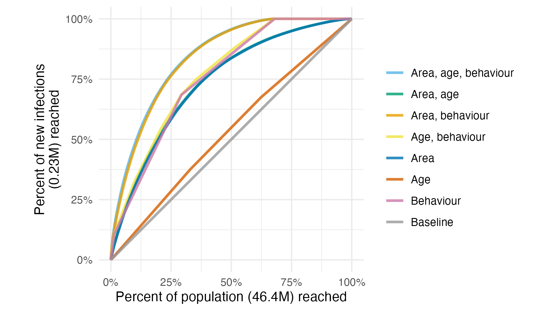
Figure 5.10: Percentage of new infections reached across all 13 countries, taking a variety of risk stratification approaches, against the percentage of at risk population required to be reached.
For any given fraction of AGYW prioritised, substantially more new infections were reached by strategies that included behavioural risk stratification. Reaching half of all expected new infections required reaching 19.4% of the population when stratifying by subnational area and age, but only 10.6% when behavioural stratification was included (Figure 5.10). The majority of this benefit came from reaching FSW, who were 1.3% of the population but 10.6% of all new infections.
Considering each country separately, on average, reaching half of new infections in each country required reaching 14.6% (range 8.7-21.8%) of the population when stratifying by area and age, reducing to 5.1% (range 2.1-13.2%) when behaviour was included. The relative importance of stratifying by age, location and behaviour varied between countries, analogous to the varying contribution of each to the total variance (Section 5.5.1.3).
5.6 Discussion
In this chapter, I estimated the proportion of AGYW who fall into different risk groups at a district level in 13 sub-Saharan African countries. These estimates support consideration of differentiated prevention programming according to geographic locations and risk behaviour, as outlined in the Global AIDS Strategy. Systematic differences in risk by age groups, and variation within and between countries, explained the large majority of variation in risk group proportions. Changes over time were negligible in the overall variation in risk group proportions. The proportion of 15-19 year olds who are sexually active, and among women aged 20-29 years, norms around cohabitation especially varied across districts and countries. This variation underscores the need for these granular data to implement HIV prevention options aligned to local norms and risk behaviours.
I considered four risk groups based on sexual behaviour, the most proximal determinant of risk. Other factors, such as condom usage or type of sexual act, may account for additional heterogeneity in risk from sexual behaviour. However, I did not include these factors in view of measurement difficulties, concerns about consistency across contexts, and the operational benefits of describing risk parsimoniously.
Sexual behaviour confers risk only when AGYW reside in geographic locations where there is unsuppressed viral load among their potential partners. I did not include more distal determinants, such as school attendance, orphanhood, or gender empowerment, as I expect their effects on risk to largely be mediated by more proximal determinants. However, to effectively implement programming, it is crucial to understand these factors, as well as the broader structural barriers and limits to personal agency faced by AGYW. Importantly, programs must ensure that intervention prioritisation occurs without stigmatising or blaming AGYW.
By considering a range of possible risk stratification strategies, I showed that successful implementation of a risk-stratified approach would allow substantially more of those at risk for infections to be identified before infection occurs. A considerable proportion of estimated new infections were among FSW, supporting the case for HIV programming efforts focused on key population groups (Baral et al. 2012). There is substantial variation in the importance of prioritisation by age, location and behaviour within each country. This highlights the importance of understanding and tailoring HIV prevention efforts to country-specific contexts. By standardising the analysis across all 13 countries, I showed the additional efficiency benefits of resource allocation between countries.
I found a geographic delineation in the proportion of women cohabiting between southern and eastern Africa, calling attention to a divide attributable to many cultural, social, and economic factors. The delineation does not represent a boundary between predominately Christian and Muslim populations, which is further north. I also note that the high numbers of adolescent girls aged 15-19 cohabiting in Mozambique is markedly different from the other countries (UNICEF 2019).
Brugh et al. (2021) previously geographically mapped AGYW HIV risk groups using biomarker and behavioural data from the most recent surveys in Eswatini, Haiti and Mozambique to define and subsequently map risk groups with a range of machine learning techniques. My work builds on Brugh et al. (2021) by including more countries, integrating a greater number of surveys, and connecting risk group proportions with HIV epidemic indicators to help inform programming.
My modelled estimates of risk group proportions improve upon direct survey results for three reasons. First, by taking a modular modelling approach, I integrated all relevant survey information from multiple years, allowing estimation of the FSW proportion for surveys without a specific transactional sex question. Second, whereas direct estimates exhibit large sampling variability at a district level, I alleviated this issue using spatio-temporal smoothing (Figure 5.11). Third, I provided estimates in all district-years, including those not directly sampled by surveys, allowing estimates to be consistently fed into further analysis and planning pipelines such as my analysis of risk group specific prevalence and incidence.
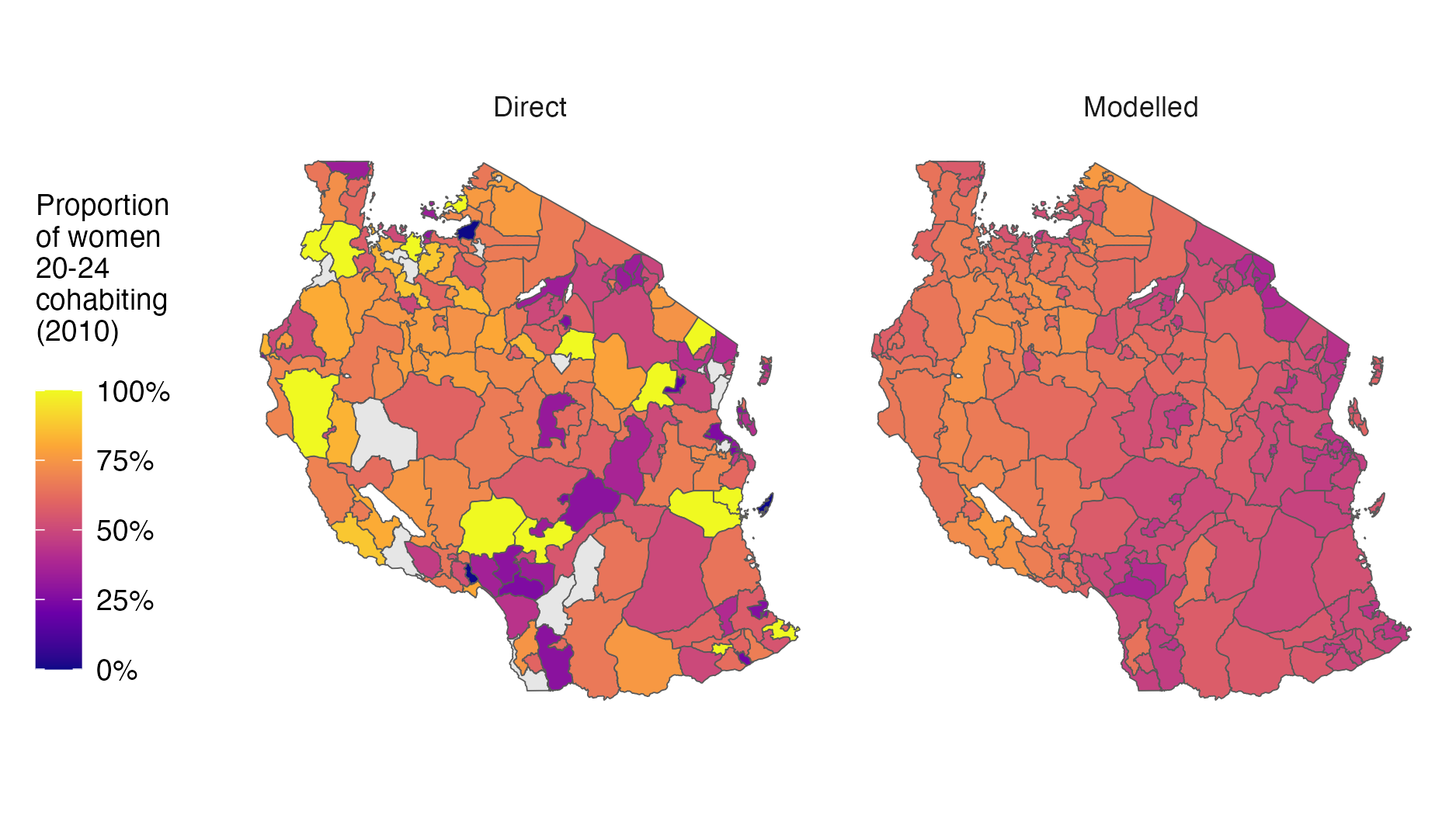
Figure 5.11: The modelled estimates display more plausible spatial smoothness than the direct estimates. In addition, missing values in the direct estimates are appropriately infilled by the model.
The final surveys included in the risk model model were conducted in 2018. The analysis may be updated with more surveys as they become available. I do not anticipate that the risk group proportions will change substantially, as I found that they did not change significantly over time.
My analysis focused on females aged 15-29 years, and could be extended to consider optimisation of prevention more broadly, accounting for new infections among adults 15-49 which occur in women 30-49 and men 15-49. Estimating sexual risk behaviour in adults 15-49 would be a crucial step toward greater understanding of the dynamics of the HIV epidemic in sub-Saharan Africa, and would allow incidence models to include stratification of individuals by sexual risk.
5.6.1 Limitations
This analysis was subject to challenges shared by most approaches to monitoring sexual behaviour in the general population (Cleland et al. 2004). In particular, under-reporting of higher risk sexual behaviours among AGYW could affect the validity of my risk group proportion estimates. Due to social stigma or disapproval, respondents may be reluctant to report non-marital partners (Nnko et al. 2004; Helleringer et al. 2011) or may bias their reporting of sexual debut (Zaba et al. 2004; Wringe et al. 2009; Nguyen and Eaton 2022). For guidance of resource allocation, differing rates of under-reporting by country, district, year or age group are particularly concerning to the applicability of my results; and, while it may be reasonable to assume a constant rate over space-time, the same cannot be said for age, where aspects of under-reporting have been shown to decline as respondents age (Glynn et al. 2011), suggesting that the elevated risks I found faced by younger women are likely a conservative estimate. If present, these reporting biases will also have distorted the estimates of infection risk ratios and prevalence ratios I used in my analysis, likely over-attributing risk to higher risk groups.
I have the least confidence in my estimates for the FSW risk group. As well as having the smallest sample sizes, my transactional sex estimates do not overcome the difficulties of sampling hard to reach groups. I inherent any limitations of the national FSW estimates (Stevens et al. 2023) which I adjust my estimates of transactional sex to match. Furthermore, I do not consider seasonal migration patterns, which may particularly affect FSW population size. More generally, I did not consider covariates potentially predictive of risk group proportions (such as sociodemographic characteristics, education, local economic activity, cultural and religious norms and attitudes), which are typically difficult to measure spatially. Identifying measurable correlates of risk, or particular settings in which time-concentrated HIV risk occurs, is an important area for further research to improve risk prioritisation and precision HIV programme delivery.
The efficiency of each stratified prevention strategy depends on the ability of programmes to identify and effectively reach those in each strata. My analysis of new infections potentially averted assumed a “best-case” scenario where AGYW of every strata can be reached perfectly, and should therefore be interpreted as illustrating the potentially obtainable benefits rather than benefits which would be obtained from any specific intervention strategy. In practice, stratified prevention strategies are likely to be substantially less efficient than this best-case scenario. Factors I did not consider include the greater administrative burden of more complex strategies, variation in difficulty or feasibility of reaching individuals in each strata, variation in the range or effectiveness of interventions by strata, and changes in strata membership that may occur during the course of a year. Identifying and reaching behavioural strata may be particularly challenging. Empirical evaluations of behavioural risk screening tools have found only moderate discriminatory ability (Jia et al. 2022), and risk behaviour may change rapidly among young populations, increasing the challenge to effectively deliver appropriately timed prevention packages. This consideration may motivate selecting risk groups based on easily observable attributes, such as attendance of a particular service or facility, rather than sexual behaviour.
In conducting this work, there was insufficient engagement with country experts or civil society organisations. As a result, in early use of the risk group tool the FSW population size estimates were met with some disagreement in Malawi. In that instance, the cause of the disagreement was external model inputs used. In future, estimates should be generated and reviewed by country teams.
5.6.2 Conclusion
I estimated HIV risk group proportions, HIV prevalences and HIV incidences for AGYW aged 15-19, 20-24 and 25-29 years at a district-level in 13 priority countries. Using these estimates, I analysed the number of infections that could be reached by prioritisation based upon location, age and behaviour. Though subject to limitations, these estimates provide data that national HIV programmes can use to set targets and implement differentiated HIV prevention strategies as outlined in the Global AIDS Strategy. Successfully implementing this approach would result in more efficiently reaching a greater number of those at risk of infection.
Among AGYW, there was systematic variation in sexual behaviour by age and location, but not over time. Age group variation was primarily attributable to age of sexual debut (ages 15-24). Spatial variation was particularly present between those who reported one cohabiting partner versus non-regular or multiple partners. Risk group proportions did not change substantially over time, indicating that norms relating to sexual behaviour are relatively static. These findings underscore the importance of providing effective HIV prevention options tailored to the needs of particular age groups, as well as local norms around sexual partnerships.